Welcome to My Blog
Security researchers take control of a brand new Mac on first Wi-Fi connection

Security researchers at the Black Hat conference in Las Vegas have demonstrated a method of taking control of a brand new Mac as it makes its first Wi-Fi connection.
A vulnerability in the way Macs handle Mobile Device Management allowed them to install unlimited Malware on the machine prior to its owner even seeing the desktop for the first time …
How to Grow: Wisdom From 6 Years of Podcasting

In this special edition of the Social Media Marketing podcast, I reveal four lessons I have picked up from 6 years of podcasting (and growing Social Media Examiner). The topics I’ll cover include how to grow anything, how to succeed via omission, how to achieve thought leadership, and my view on competition. I’ll also share […]
The post How to Grow: Wisdom From 6 Years of Podcasting appeared first on Social Media Examiner.
from Social Media Examiner https://ift.tt/2vUkL6o
via socialmediaexaminer
How to Add a Text Box in Google Docs [FAQ]
A text box is an effective way to draw attention to important information on a page, or organize your thoughts visually.
Adding a text box to a Google Doc can also make your document look more formal and professional — which is particularly important if you’re sharing the Doc with colleagues.
If you need to differentiate a set of text for your next marketing meeting notes or brainstorming session, you’ll need to know how to add a text box in Google Docs. Fortunately, it’s incredibly easy to do. In fact, it should take less than a minute once you get the hang of it. Here’s how.
How to Add a Text Box in Google Docs
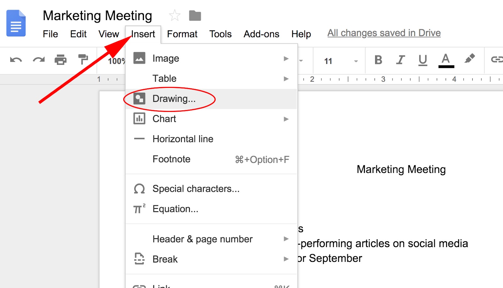
1. Go to “Insert” and then click “Drawing … “.
2. Within the Drawing tool, click the “Text box” (it’s the box in the tool bar with a “T” in the middle).

3. Draw your desired text box shape. Then, type your text into the box.

4. In the toolbar, you’ll see a paint bucket. Click that to change the color in your text box, or text box border, if you want.
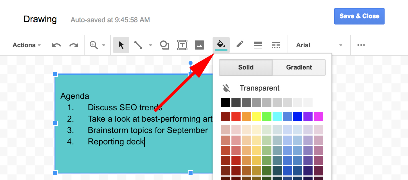
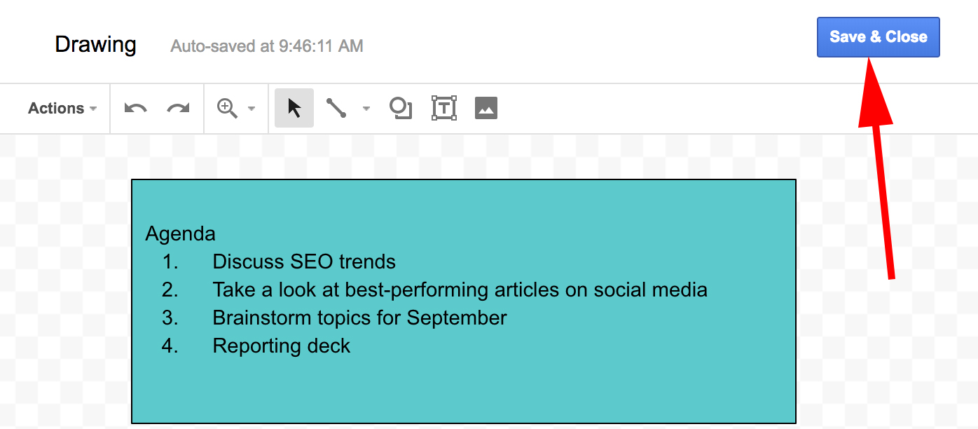
5. When you’re happy with your text box, click “Save & Close”.
6. And voila! Your text box is instantly placed in your Google Doc. If you want to move it around, simply drag it or pull the corners to change the size.

That’s it! Check out our “Ultimate Guide to Google Docs” next, if you’re looking for a more in-depth dive into the ins and outs of Google Docs.

After stint at Tesla, Doug Field returns to Apple to work on Project Titan w/ Bob Mansfield

After leaving in 2013 to join Tesla, Doug Field has now made his way back to Apple. As noted in a report from Daring Fireball, Field is returning to Apple to work alongside Bob Mansfield on Apple’s Project Titan car team…
Marantz begins rolling out AirPlay 2 support to compatible audio accessories

Back in May, Apple revealed the full list of third-party speakers slated to receive updates with AirPlay 2 support. Now, one of the first manufacturers has started rolling out updates to their line of audio accessories…
iPhone & iPad: How to change language and region

iOS lets users change their language and region, in case you decide to move away to a different country, or if you’d like to simply change the date format.
How to Sort in Excel: A Simple Guide to Organizing Data
When it comes to Excel, here’s a good rule to live by: If you find yourself doing something manually, there’s probably an easier way.
Whether you’re trying to remove duplicates, do simple calculations, or sort your data, you can almost always find a workaround that’ll help you get it done with just a click (or two) of a button.
But if you’re not a power user, it’s easy to overlook these shortcuts. And before you know it, something as simple as organizing a list of names in alphabetical order can suck up a ton of your time.

Luckily, there is a workaround for that. In fact, there are a few different ways to use Excel’s sorting feature that you may not know about. Let’s check them out below, starting with the basics.
How to Sort in Excel
- Highlight the rows and/or columns you want sorted.
- Navigate to “Data” along the top and select “Sort.”
- If sorting by column, select the column you want to order your sheet by.
- If sorting by row, click “Options” and select “Sort left to right.”
- Choose what you’d like sorted.
- Choose how you’d like to order your sheet.
- Click “OK.”
For this first set of instructions, we’ll be using Microsoft Excel 2017 for Mac. But don’t worry — while the location of certain buttons might be different, the icons and selections you have to make are the same across most earlier versions of Excel.
1. Highlight the rows and/or columns you want sorted.
To sort a range of cells in Excel, first click and drag your cursor across your spreadsheet to highlight all of the cells you want to sort — even those rows and columns whose values you’re not actually sorting by.
For example, if you want to sort column A, but there’s data associated with column A in columns B and C, it’s important to highlight all three columns to ensure the values in Columns B and C move along with the cells you’re sorting in Column A.
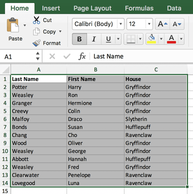
In the screenshot below, we’re going to sort this sheet by the last name of Harry Potter characters. But the first name and house of each person needs to go with each last name that gets sorted, or each column will become mismatched when we finish sorting.
2. Navigate to ‘Data’ along the top and select ‘Sort.’
Once all the data you want to sort is highlighted, select the “Data” tab along the top navigation bar (you can see this button on the top-right of the screenshot in the first step, above). This tab will expand a new set of options beneath it, where you can select the “Sort” button. The icon has an “A-Z” graphic on it, as you can see below, but you’ll be able to sort in more ways than just alphabetically.

3. If sorting by column, select the column you want to order your sheet by.
When you hit the “Sort” button, shown above, a window of settings will appear. This is where you can configure what you’d like sorted and how you’d like to sort it.
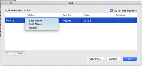
If you’re sorting by a specific column, click “Column” — the leftmost dropdown menu, shown below — and select the column whose values you want to be your sorting criteria. In our case, it’ll be “Last Name.”
4. If sorting by row, click ‘Options’ and select ‘Sort left to right.’
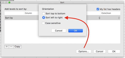
If you’d rather sort by a specific row, rather than a column, click “Options” on the bottom of the window and select “Sort left to right.” Once you do this, the Sort settings window will reset and ask you to choose the specific “Row” you’d like to sort by in the leftmost dropdown (where it currently says “Column”).
This sorting system doesn’t quite make sense for our example, so we’ll stick with sorting by the “Last Name” column.
5. Choose what you’d like sorted.
You don’t just have to sort by the value of each cell. In the middle column of your Sort settings window, you’ll see a dropdown menu called “Sort On.” Click it, and you can choose to sort your sheet by different characteristics of each cell in the column/row you’re sorting by. These options include cell color, font color, or any icon included in the cell.
6. Choose how you’d like to order your sheet.
In the third section of your Sort settings’ window, you’ll see a dropdown bar called “Order.” Click it to select how you’d like to order your spreadsheet.
By default, your Sort settings window will suggest sorting alphabetically (which we’ll show you shortcuts for in the next process below). But you can also sort from Z to A, as well as by a custom list. While you can create your own custom list, there are a few preset lists you can sort your data by right away. We’ll talk more about how and why you might sort by custom list in a few minutes.
To Sort by Number
If your spreadsheet includes a column of numbers, rather than letter-based values, you can also sort your sheet by these numbers. To do that, you’ll select this column in the leftmost “Columns” dropdown menu. This will change the options in the “Order” dropdown bar so that you can sort from “Smallest to Largest” or “Largest to Smallest.”
7. Click ‘OK.’
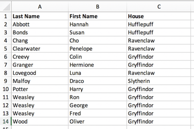
Click “OK,” in your Sort settings window, and you should see your list successfully sorted according to your desired criteria. Here’s what our Harry Potter list now looks like, organized by last name in alphabetical order:
How to Alphabetize in Excel
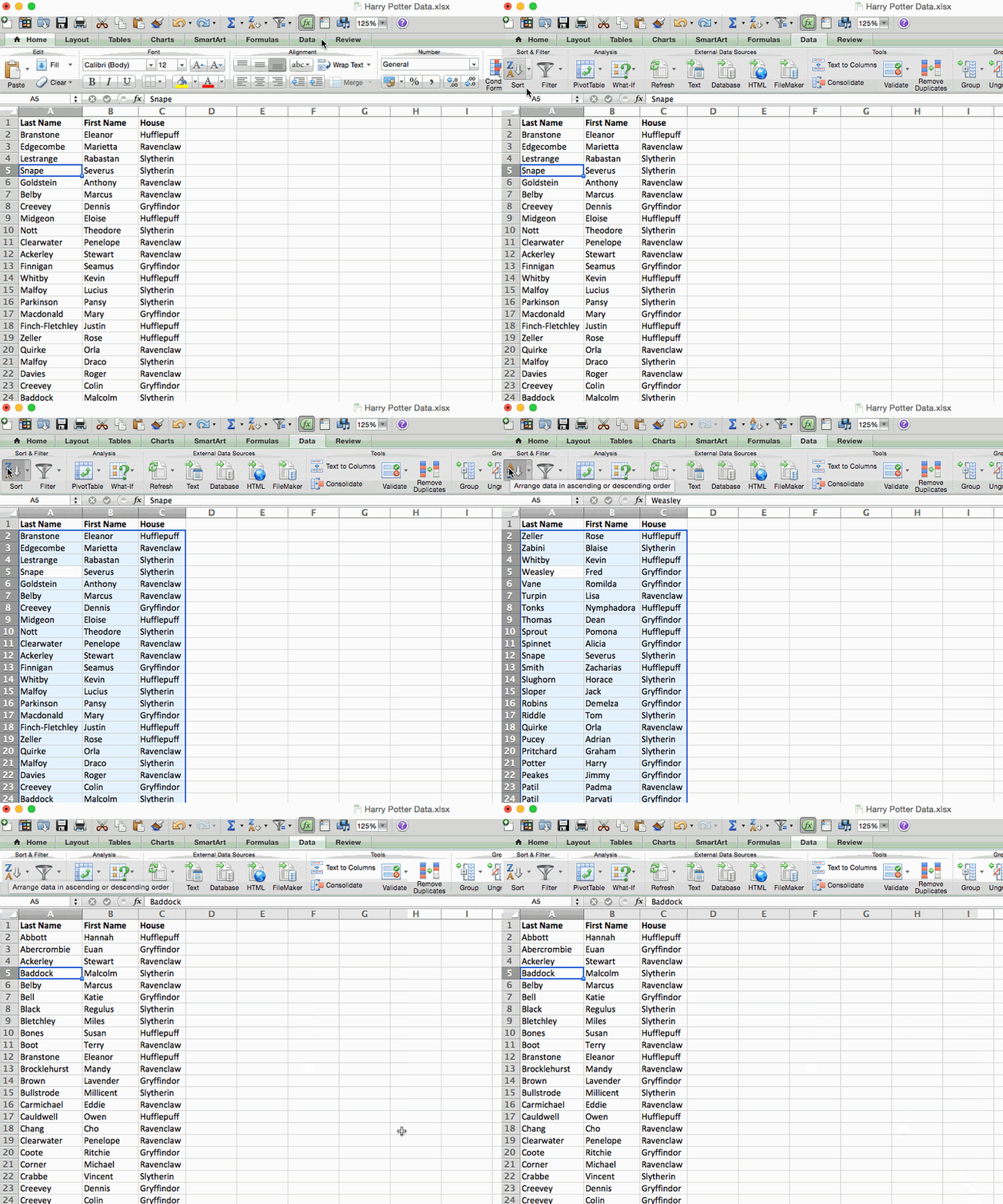
To alphabetize in Excel, highlight a cell in the column you want to sort by. Click the Data tab along the top navigation, and you’ll see buttons for sorting in forward or reverse alphabetical order. Clicking either button will order your sheet according to the column of the cell you first highlighted.
Sometimes you may have a list of data that has no organization whatsoever. Maybe you exported a list of your marketing contacts or blog posts. Whatever the case may be, you might want to start by alphabetizing the list — and there’s an easy way to do this that doesn’t require you to follow each step outlined above.
To Alphabetize on a Mac
- Select a cell in the column you want to sort.
- Click on the “Data” tab in your toolbar and look for the “Sort” option on the left.
- If the “A” is on top of the “Z,” you can just click on that button once. If the “Z” is on top of the “A,” click on the button twice. Note: When the “A” is on top of the “Z,” that means your list will be sorted in alphabetical order. However, when the “Z” is on top of the “A,” that means your list will be sorted in reverse alphabetical order.
To Alphabetize on a PC
- Select a cell in the column you want to sort.
- Click on the “Data” tab in your toolbar. You will see Sort options in the middle.
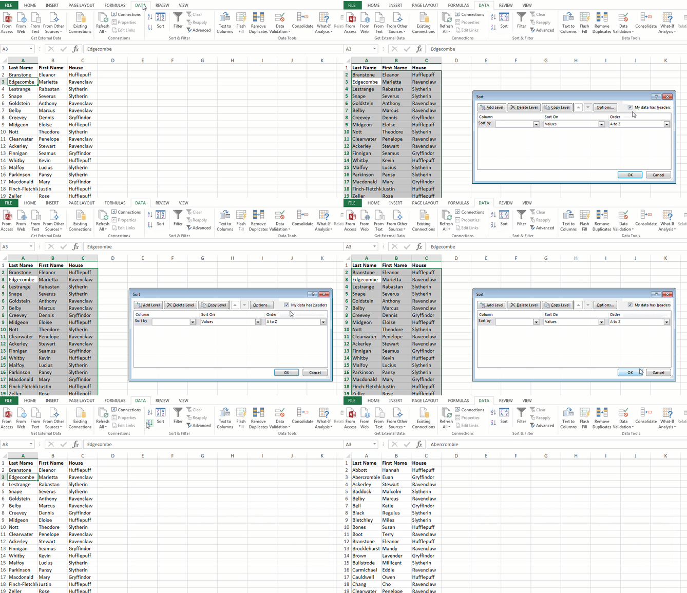
- Click on the icon above the word “Sort.” A pop-up will appear: If you have headers, make sure “My list has headers” is checked. If it is, click “Cancel.”
- Click on the button that has the “A” on top and the “Z” on the bottom with an arrow pointing down. That will sort your list alphabetically from “A” to “Z.” If you want to sort your list in reverse alphabetical order, click on the button that has the “Z” on top and the “A” on the bottom.
Sorting Multiple Columns
Sometimes you don’t just want to sort one column, but you want to sort two. Let’s say you want to organize all of your blog posts that you have in a list by the month they were published. First, you’d want to organize them by date, and then by the blog post title or URL.
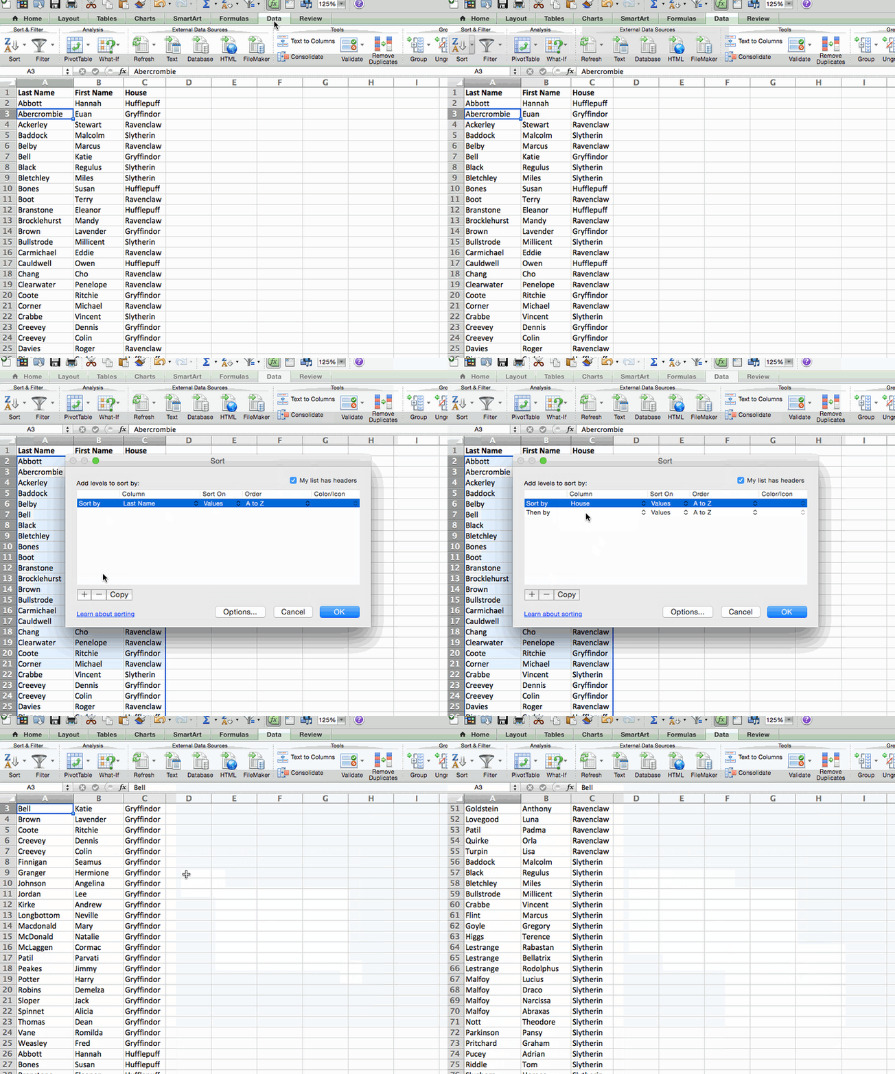
In this example, I want to sort my list first by house, and then by last name. This would give me a list organized by each house, but also alphabetized within each house.
To Sort Multiple Columns on a Mac
- Click on the data in the column you want to sort.
- Click on the “Data” tab in your toolbar and look for the “Sort” option on the left.
- Click on the small arrow to the left of the “A to Z” Sort icon. Then, select “Custom Sort” from the menu.
- A pop-up will appear: If you have headers, make sure “My list has headers” is checked.
- You will see five columns. Under “Column” select the first column you want to sort from the dropdown menu. (In this case, it is “House.”)
- Then, click on the “+” sign at the bottom left of the pop-up. Under where it says “Column,” select “Last Name” from the dropdown.
- Check the “Order” column to make sure it says A to Z. Then click “OK.”
- Marvel at your beautiful organized list.
To Sort Multiple Columns on a PC
- Click on the data in the column you want to sort.
- Click on the “Data” tab in your toolbar. You will see “Sort” options in the middle.
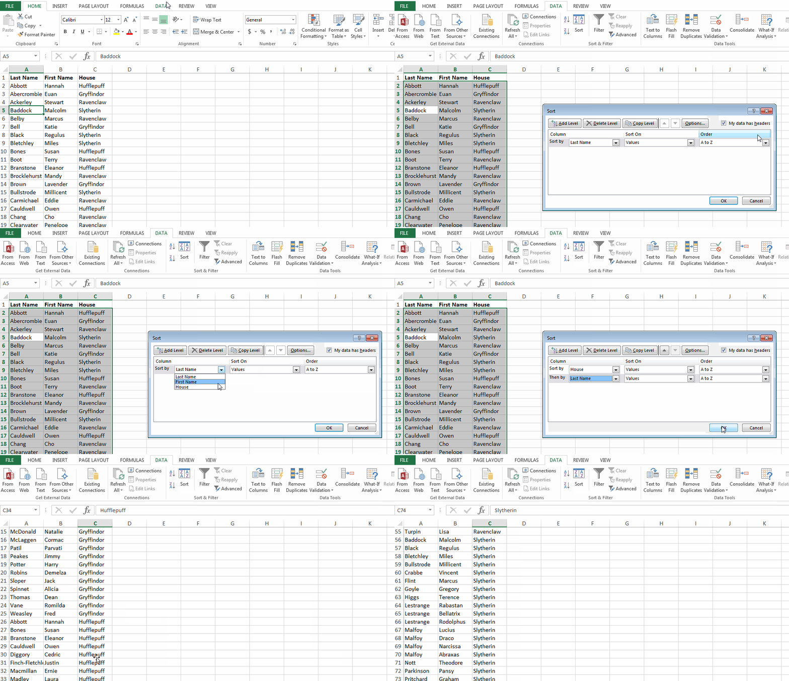
- Click on the icon above the word “Sort.” You will see a pop-up appear. Make sure “My data has headers” is checked if you have column headers.
- You will see three columns. Under “Column” select the first column you want to sort from the dropdown menu. (In this case, it is “House.”)
- Then click on “Add Level” at the top left of the pop-up. Under where it says “Column” select “Last Name” from the dropdown.
- Check the “Order” column to make sure it says A to Z. Then click “OK.”
- Marvel at your beautiful organized list.
Sorting in Custom Order
Sometimes you don’t want to sort by A to Z or Z to A. Sometimes you want to sort by something else, such as months, days of the week, or some other organizational system.
In situations like this, you can create your own custom order to specify exactly the order you want the sort. (It follows a similar path to multiple columns but is slightly different.)
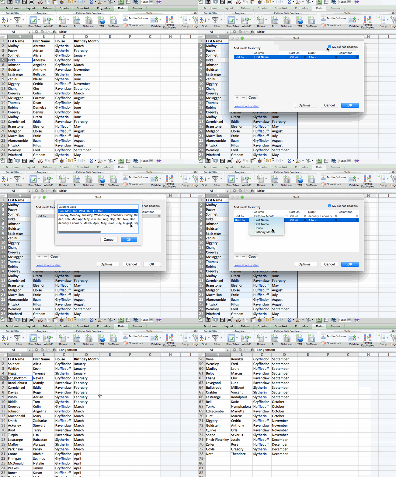
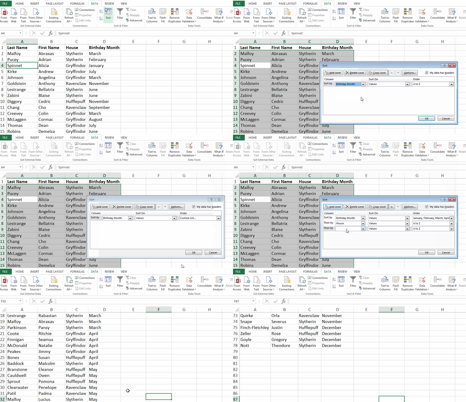
Let’s say we have everyone’s birthday month at Hogwarts, and we want everyone to be sorted first by Birthday Month, then by House, and then by Last Name.
To Sort in Custom Order on a Mac
- Click on the data in the column you want to sort.
- Click on the “Data” tab in your toolbar. You will see “Sort” all the way to the left.
- Click on the small arrow to the left of the “A to Z” Sort icon. Then, select “Custom Sort” from the menu.
- A pop-up will appear: If you have headers, make sure “My list has headers” is checked.
- You will see five columns. Under “Column,” select the first column in your spreadsheet you want to sort from the dropdown menu. In this case, it is “Birthday Month.”
- Under the “Order” column, click on the dropdown next to “A to Z.” Select the option for “Custom List.”
- You will see a couple of options (month and day). Select the month list where the months are spelled out, as that matches the data. Click “OK.”
- Then click on the “+” sign at the bottom left of the pop-up. Under “Column,” select “House” from the dropdown.
- Click on the “+” sign at the bottom left again. Under “Column,” select “Last Name” from the dropdown.
- Check the “Order” column to make sure “House” and “Last Name” say A to Z. Then click “OK.”
- Marvel at your beautiful organized list.
To Sort in Custom Order on a PC
- Click on the data in the column you want to sort.
- Click on the “Data” tab in your toolbar. You will see “Sort” options in the middle.
- Click on the icon above the word “Sort.” You will see a pop-up appear: If you have headers, make sure “My list has headers” is checked.
- You will see three columns. Under “Column,” select the first column you want to sort from the dropdown. In this case, it is “Birthday Month.”
- Under the “Order” column, click on the dropdown next to “A to Z.” Select the option for “Custom List.”
- You will see a couple of options (month and day), as well as the option to create your own custom order. Select the month list where the months are spelled out, as that matches the data. Click “OK.”
- Then, click on “Add Level” at the top left of the pop-up. Under “Column,” select “House” from the dropdown.
- Click on the “Add Level” button at the top left of the pop-up again. Under “Column,” select “Last Name” from the dropdown.
- Check the “Order” column to make sure “House” and “Last Name” say A to Z. Then click “OK.”
- Marvel at your beautiful organized list.
Sorting a Row
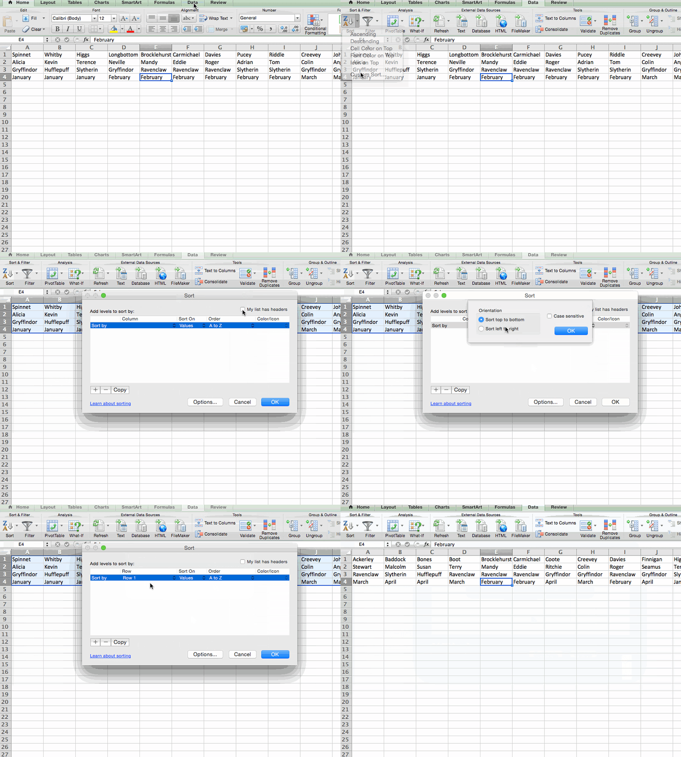
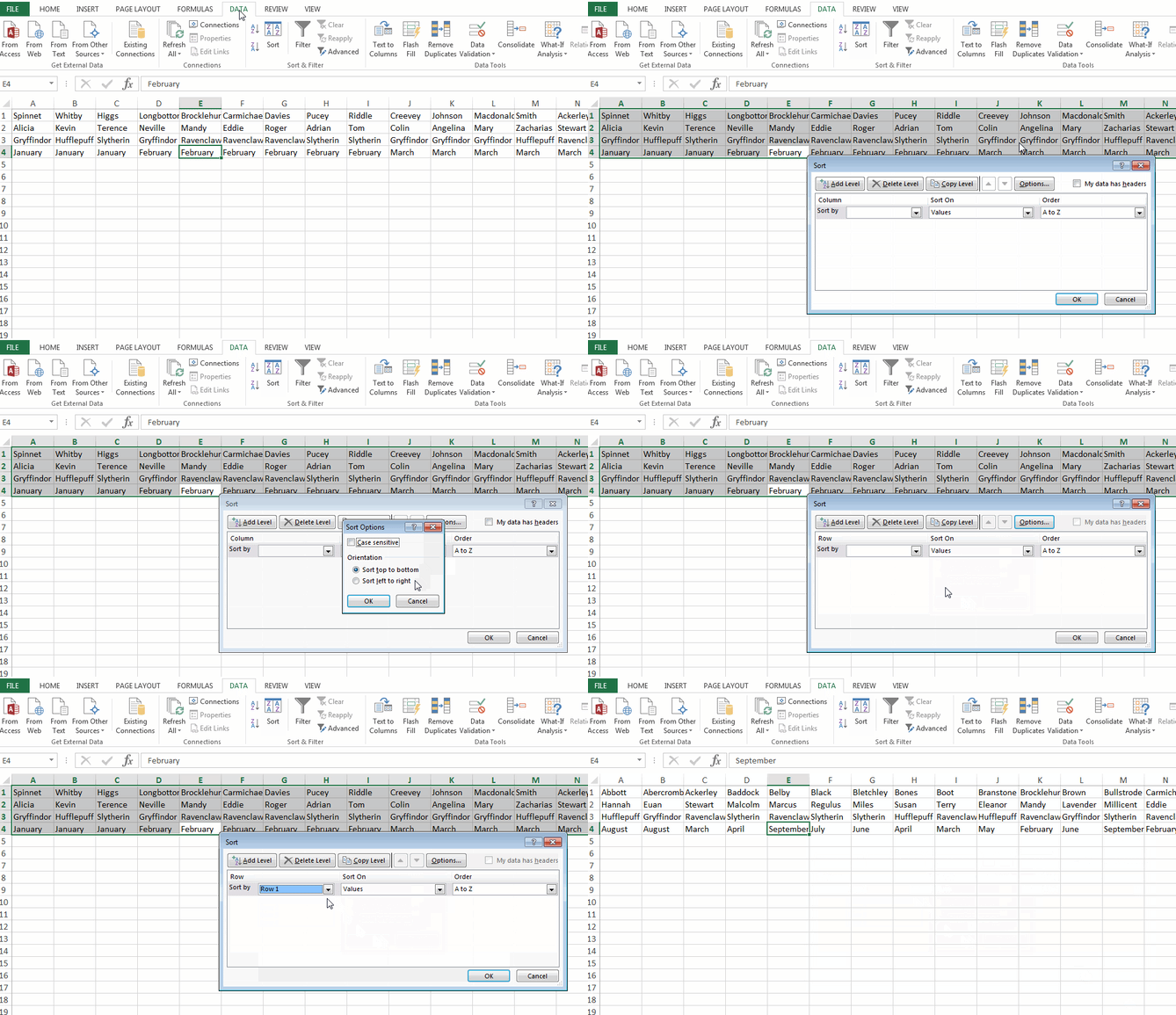
Sometimes your data may appear in rows instead of columns. When that happens you are still able to sort your data with a slightly different step.
To Sort a Row on a Mac
- Click on the data in the row you want to sort.
- Click on the “Data” tab in your toolbar. You will see “Sort” all the way to the left.
- Click on the small arrow to the left of the “A to Z” Sort icon. Then, select “Custom Sort” from the menu.
- A pop-up will appear: Click on “Options” at the bottom.
- Under “Orientation” select “Sort left to right.” Then, click “OK.”
- You will see five columns. Under “Row,” select the row number that you want to sort from the dropdown. (In this case, it is Row 1.) When you are done, click “OK.”
To Sort a Row on a PC
- Click on the data in the row you want to sort.
- Click on the “Data” tab in your toolbar. You will see “Sort” options in the middle.
- Click on the icon above the word “Sort.” You will see a pop-up appear.
- Click on “Options” at the bottom.
- Under “Orientation” select “Sort left to right.” Then, click “OK.”
- You will see three columns. Under “Row,” select the row number that you want to sort from the dropdown. (In this case, it is Row 1.) When you are done, click “OK.”
Sort Your Conditional Formatting
If you use conditional formatting to change the color of a cell, add an icon, or change the color of a font, you can actually sort by that, too.
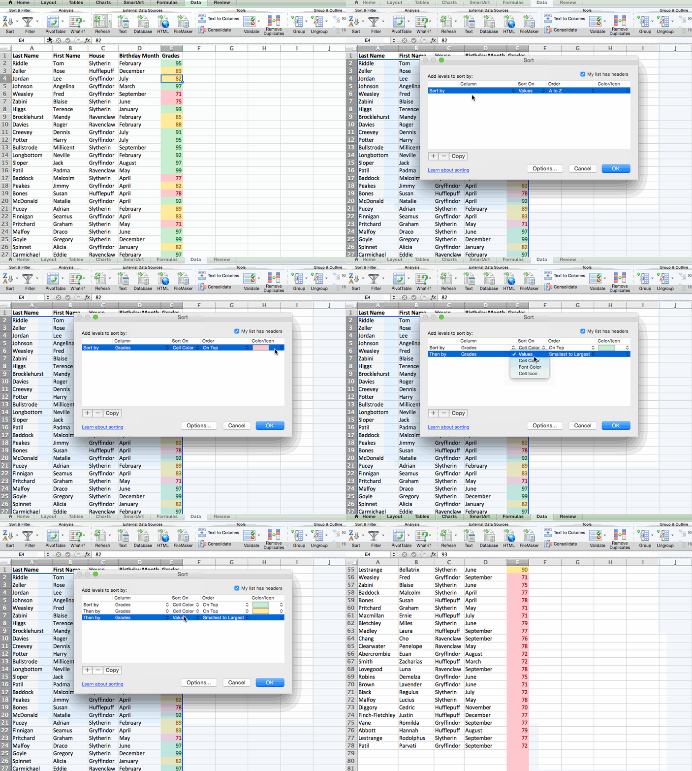
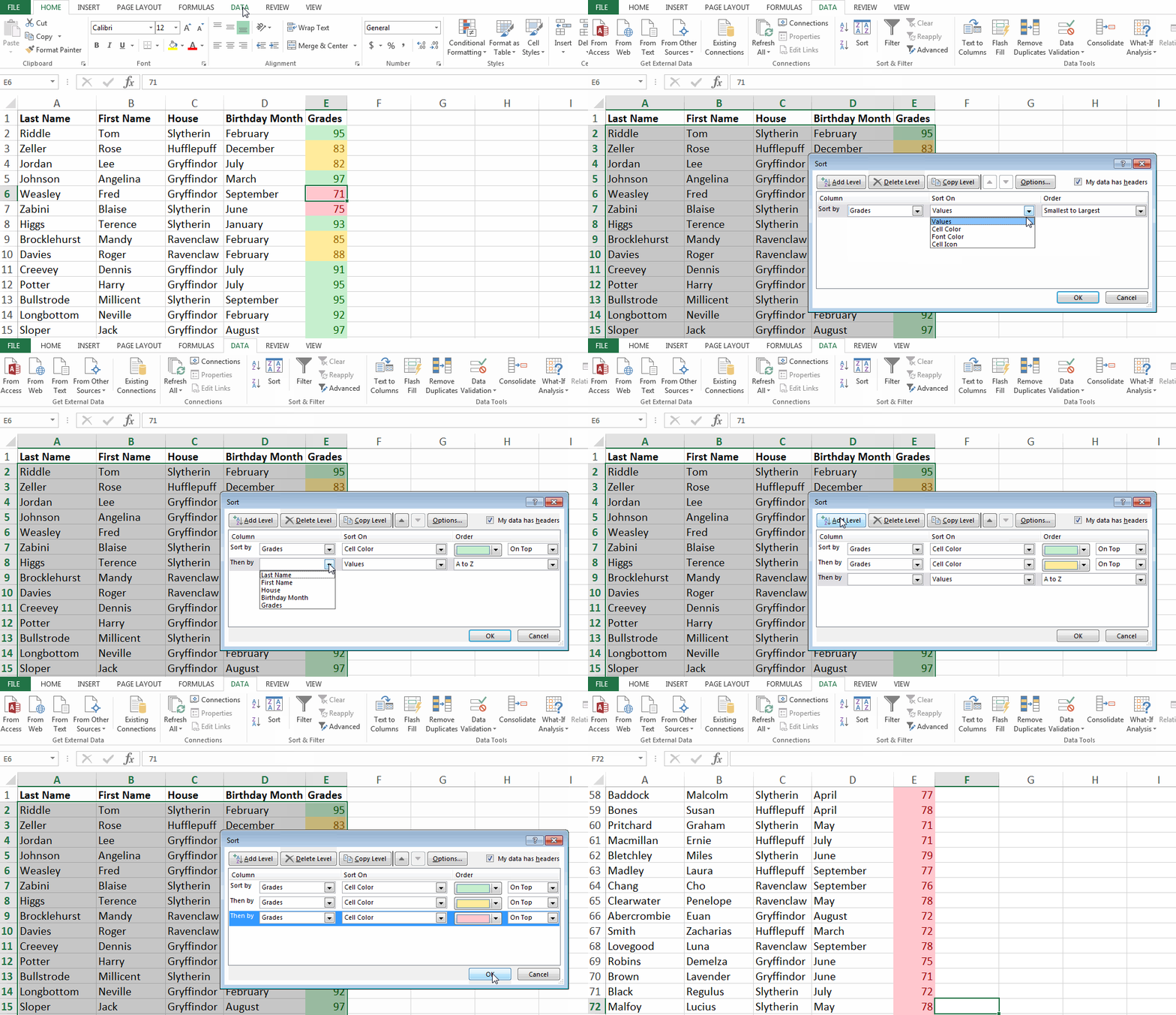
In the example below, I’ve used colors to signify different grade ranges: If they have a 90 or above, the cell appears green. Between 80-90 is yellow. Below 80 is red. Here’s how you’d sort that information to put the top performers at the top of the list. I want to sort this information so that the top performers are at the top of the list.
To Sort Conditional Formatting on a Mac
- Click on the data in the row you want to sort.
- Click on the “Data” tab in your toolbar. You will see “Sort” all the way to the left.
- Click on the small arrow to the left of the “A to Z” Sort icon. Then, select “Custom Sort” from the menu.
- A pop-up will appear: If you have headers, make sure “My list has headers” is checked.
- You will see five columns. Under “Column,” select the first column you want to sort from the dropdown. In this case, it is “Grades.”
- Under the column that says “Sort On,” select “Cell Color”.
- In the last column that says “Color/Icon,” select the green bar.
- Then click on the “+” sign at the bottom left of the pop-up. Repeat steps 5-6. Instead of selecting green under “Color/Icon,” select the yellow bar.
- Then click on the “+” sign at the bottom left of the pop-up. Repeat steps 5-6. Instead of selecting green under “Color/Icon,” select the red bar.
- Click “OK.”
To Sort Conditional Formatting on a PC
- Click on the data in the row you want to sort.
- Click on the “Data” tab in your toolbar. You will see “Sort” options in the middle.
- Click on the icon above the word “Sort.” A pop-up will appear: If you have headers, make sure “My list has headers” is checked.
- You will see three columns. Under “Column” select the first column you want to sort from the dropdown. In this case, it is “Grades.”
- Under the column that says “Sort On,” select “Cell Color”.
- In the last column that says “Order,” select the green bar.
- Click on “Add Level.” Repeat steps 4-5. Instead of selecting green under “Order,” select the yellow bar.
- Click on “Add Level” again. Repeat steps 4-5. Instead of selecting yellow under “Order,” select the red bar.
- Click “OK.”
There you have it — all the possible ways to sort in Excel. Ready to sort your next spreadsheet? Start by grabbing nine different Excel templates below, then use Excel’s sorting function to organize your data as you see fit.



MTA official allegedly stole $60K from taxpayers through iPhone ‘procurmenet-and-resale’ scheme

A former Metropolitan Transportation Authority official has been indicted on accusations of buying some $60,000 worth of iPhones with taxpayer money – only to resell them and pocket the money…
iPhone X outperforms Samsung’s brand new 6.4-inch Galaxy Note 9

Earlier today, Samsung officially unveiled its brand new (and oft-leaked) Galaxy Note 9 with a 6.4-inch display. While Samsung touts the device’s Qualcomm Snapdragon 845 chipset and 6GB or 8GB of RAM under-the-hood, but earlier benchmarks show the device is still outperformed by the iPhone X…
Apple orders straight-to-series comedy featuring Charlie Day & Rob McElhenney

Apple continues its efforts to expand its catalog of original content today. While everything is still behind the scenes, and nothing has been officially announced yet, the company has been on a roll, working hard to add more to its catalog seemingly every week…
Mac: How to change your language and region

Do you use your Mac in multiple languages? Are you moving to a new country or would like to change your Mac’s region setting? Follow along below…
Apple Pay has over 252M users globally, more popular internationally than US

Following a positive outlook on Apple’s earnings call last week, Loup Ventures is out today with an in-depth look at the state of Apple Pay. Currently, Loup Ventures estimates that just 20 percent of global smartphone users rely on their phone as a wallet, but it expects that number to rise to 80 percent…
These are the new emoji candidates for 2019, including service dog, couple variants, more

The Unicode Consortium has released an update today on the emoji that could be released next year. Candidates include a service dog, deaf person, and over 50 new combinations of couples holding hands.
9to5Mac Daily: August 9, 2018

Listen to a recap of the top stories of the day from 9to5Mac. 9to5Mac Daily is available on iTunes and Apple’s Podcasts app, Stitcher, TuneIn, Google Play, or through our dedicated RSS feed for Overcast and other podcast players.
Twitter for iPhone and iPad dropping iOS 9 support in next update

Twitter for iPhone and iPad will soon drop support for older devices running iOS 9, according to the release notes for today’s app update. Starting with the next version of Twitter for iOS, users will need to be running iOS 10 or higher to continue receiving app updates and new features.
Angela Ahrendts discusses intuitive leadership, challenges of building timeless brands, more in Global Leadership Summit interview

Today at the 2018 Global Leadership Summit in South Barrington, Illinois, Apple’s SVP of Retail Angela Ahrendts spoke about her leadership journey during an interview with author and coach John Maxwell.
Broadcast to 125,000 individuals both on-site and across 75 host locations, at one of which 9to5Mac attended, the wide-ranging interview shed light on Ahrendts’s leadership strategy, Apple’s goal of enriching lives, and the challenges of building a timeless brand.
Apple pushes GiveBack program with trade-ins now worth instant credit toward new iPhone, iPad, Apple Watch, Mac

Apple rebranded its reuse and recycling trade-in program earlier this year as “Apple GiveBack.” Now, customers buying new devices on Apple’s website can use a trade-in to instantly offset the cost.