
Welcome to My Blog
Japanese watchdog says Apple may have broken antitrust rules but won’t be punished

An investigation spanning almost two years has concluded that Apple ‘may’ have breached antitrust rules in Japan by forcing carriers to sell iPhones at an apparent discount …
How to Create a Messenger Bot Sequence for Your Live Video or Webinar

Do you use webinars or live video in your marketing? Wondering how to improve registrations and attendance? In this article, you’ll discover how to build a Facebook Messenger bot sequence to register and remind attendees of your live online events. Why Use Messenger Bots With Live Events? Live video streaming is a fun, engaging way […]
The post How to Create a Messenger Bot Sequence for Your Live Video or Webinar appeared first on Social Media Examiner.
from Social Media Examiner https://ift.tt/2NGazq5
via socialmediaexaminer
The Dunning Kruger Effect: Why Your Coworkers Believe They’re Way Smarter Than They Actually Are
If you’ve ever been a manager, you know how frustrating the Dunning Kruger effect can be.
Let’s say you work at a software company, and you need to give Karen, your newest software developer, a performance review. Karen’s exceptionally good at developing code, but she lacks a few critical programming skills. That’s okay — you recognized this skill gap before hiring her, and set up training sessions for this reason.
But when you mention Karen’s programming skill gap to her, her reaction baffles you: “What are you talking about? I’m exceptionally skilled at programming. I don’t need training — in fact, I’m one of the best programmers on your team.”
You’re surprised. Not only is Karen unable to recognize her weakness, but she overestimates her skill in comparison to others, believing herself to be better than some of your best developers. Her lack of knowledge on the subject makes her unable to see her own errors — this is known as the Dunning Kruger effect.
Dunning Kruger Effect
The Dunning Kruger Effect is a pyschological phenomenon in which people of the lowest ability in a subject rate themselves as most competent, compared to others. Ironically, people who lack the most knowledge on a topic also lack the ability to recognize their own mistakes and errors, making them exceptionally confident and biased self-evaluators. They are also unable to fairly judge other people’s performance.
The Dunning Kruger effect, first coined by David Dunning and Justin Kruger in 1999, is a cognitive bias that influences everyone’s perception of their own abilities. Simply put, people are unreliable resources for evaluating their own skills and shortcomings.
However, the Dunning Kruger effect gets slightly more complex than that. People like Karen, with the lowest levels of competency in a subject, often rate themselves highest in terms of expertise. Dunning and Kruger explain this as a double-curse — Karen makes mistakes because she’s not competent in a skill, but that same incompetency blinds her from seeing any errors in her work. In short, she’s not skilled enough in a particular area to see she’s not the best at it. She also misjudges other people’s abilities, assuming she knows more than most of her colleagues.
Meanwhile, true experts often underrate themselves — they’re so knowledgable on the subject, they can see how much they don’t know.
Here, we’ll dive into a few key research findings to exemplify this effect in-action. We’ll also explore a few potential solutions, so you can help any Karens — or any other colleagues on your team who suffer from the Dunning Kruger effect — fairly judge her performance moving forward.
Dunning Kruger Effect Examples
There have been numerous research studies over the years to support the notion that people misjudge their own adequacy — and, that the poorest performers are least accurate about their own skills. Let’s look at three examples now.
Example One: Debate Skills
Ehrlinger et al.’s 2008 study examined students in a collegiate debate tournament. As you might’ve guessed, students performing in the lowest 25% grossly overestimated their skills — they guessed they’d won almost 60% of their matches. In fact, they’d won about 22% of them.
The lowest performers weren’t simply overcompensating for a lack of skill, or boosting their confidence to hide their insecurities. Instead, they were genuinely unaware of their incompetence — the debaters performing in the lowest 25% had the least knowledge of debating, so they were unable to accurately judge their own performance. They weren’t biased judges. They were simply uninformed ones.
The results from this study translates to plenty of real-world examples. If you’ve extensively studied marketing, you might be shocked to hear how your colleague mis-evaluates the results from your company’s new marketing campaign. He might take a look at the staggeringly-low numbers and say, “Looks good to me,” simply because he doesn’t have the skillset to understand how to read SEO analytics — and, without that skillset at all, he believes himself to be above-average.
Example Two: Logical Reasoning Skills
In 1999, Dunning and Kruger published their initial research on the Dunning Kruger effect, called, “Unskilled and unaware of it: how difficulties in recognizing one’s own incompetence lead to inflated self-assessments.” To conduct their research, they looked at people’s self-perceptions in regards to humor, logical reasoning, and grammar.
In particular, we’ll look at study two, which focuses on logical reasoning. In the study, 45 Cornell University undergraduates were asked to complete a 20-item logical reasoning test. They were then asked to evaluate their ability and test performance — first, by providing a “general logical reasoning ability” percentile ranking compared to classmates, and second, by providing an estimated test score compared to classmates. They were also asked to guess how many test scores they got correct.
As theorized, the students in the lowest 12th percentile estimated their “general logical reasoning ability” fell closer to the 68th percentile in the class, and believed their test scores fell at the 62nd percentile. They also thought they’d answered 14.2 problems correctly (on average), when in reality, their mean score was 9.6.
Ultimately, the lowest scorers believed themselves to be above-average performers. On the flip side, the top 86th percentile students drastically underestimated themselves, estimating their general ability fell almost 20 points below, around the 68th percentile.
Have you ever heard someone really good at public speaking sigh and say, “That went terribly”? They probably aren’t just acting humble — if they’re a true expert, they likely underestimate their performance in comparison to those around them.
Example Three: Emotional Intelligence
In our prior examples, we’ve seen how the Dunning Kruger effect influences a person’s perception of their logical skills — but what about other aspects of a person’s personality, like emotional intelligence?
Sheldon, Ames, and Dunning explored emotional intelligence in relation to the Dunning Kruger effect in their 2010 study. While they conducted three separate studies, we’ll focus on the first one, which required 157 masters students to complete a Mayer-Salovey Caruso Emotional Intelligence Test. Participants were given an extensive description of EI and then asked to estimate their percentile ranking on a scale from zero to 100. They also needed to estimate their score on the MSCEIT.
As you might’ve guessed, participants who scored lowest, at the 10th percentile for emotional intelligence, overstimated their EI by 63 to 69 percentile points, and believed their MSCEIT performance to be 62 to 63 points higher than it was.
On the contrary, top performers, in the 90th percentile for EI, underestimated their EI score by five to 20 points.
This example is critical for recognizing the Dunning Kruger effect is not simply related to raw logic-based skill. Instead, it biases other aspects of our lives, including social interactions. Emotional intelligence is key to becoming a better co-worker and leader, and incorrectly assuming you’ve got high EI could be detrimental to your long-term career growth.
Consider taking an emotional intelligence test, or another personality test, to fairly judge your strengths and weaknesses.
Dunning Kruger Effect Potential Solutions
Solution One: Offer Resources to Rectify Your Colleague’s Self-Perceptions
If low performers overestimate their ability in a skill because they don’t have the knowledge to fairly evaluate their performance, a solution could be to provide those low performers with the resources and knowledge necessary to accurately judge their own performances.
During their original 1999 study, Dunning and Kruger tested this hypothesis by asking participants in study four to complete a number of Wason selection tasks (which is meant to evaluate logical reasoning skills). Afterwards, they provided roughly half the participants with a training session on how to solve Wason tasks, and then asked them to re-evaluate how well they’d done.
Overall, bottom quartile performers who received the training session became better and more accurate judges of their own abilities. Before the training, they’d ranked their ability around the 55th percentile, estimated their test performance around the 51st percentile, and reported answering 5.3 problems correctly.
After the training, these same bottom performers re-ranked their ability around the 44th percentile, estimated their test performance around the 32nd percentile, and reported answering only one problem correctly.
If you’re dealing with a colleague who can’t see how badly she’s performing, perhaps it’s because she doesn’t have the tools or training necessary to see her mistakes. Rather than explaining her mistakes and hoping she’ll get it, maybe you need to go further and offer training resources to re-calibrate how she critiques her skills.
For instance, perhaps your colleague Karen’s programming inadequacy is due to a lack of knowledge of Java Script — her background in coding leads her to believe she intuitively understands Java Script, but she can’t see how programming differs from code. If this is the case, offering a free training on Java Script could show Karen how much she needs to learn, and how to better evaluate her performance.
Solution Two: Provide Feedback Sessions
When a new colleague joins your team, she carries with her a list of preconceived notions of her strengths and weaknesses — but studies have proven people’s perception of their skills are only weakly correlated to their actual performance (Mabe and West, 1982). This makes it difficult for people to fairly evaluate their own abilities — if I believe I’m an exceptionally strong writer, and I’m given a test labelled, “Writing Rules,” I’m going to speed through the test and assume all my answers are correct, and it will be harder to accept objective feedback to the contrary.
On the other hand, if I’m given a test labelled “Math Rules,” and I’m not personally invested in the subject, I’m a better self-evaluator and will more fairly judge my own performance.
However, I could be wrong about my own skills — maybe I’m better at math than I am at writing, in which case, my evaluations are biased from the get-go.
A Ehrlinger and Dunning study from 2003 tested this same concept — they provided participants with a 10-item test and either described it as an “abstract reasoning” test or as a “computer programming skills” test. The participants had already described themselves as exceptionally strong in abstract reasoning, but admitted no knowledge of computer programming. As expected, participants who believed they’d taken an “abstract reasoning” test scored themselves 12% more favorably than when the test was labelled “computer programming”.
While there are no easy solutions to this, it’s important to take into consideration. Arming your colleagues with the knowledge that they are biased judges of their own performance could be a strong initial step. Perhaps you want to conduct a feedback session, in which you teach colleagues how to openly accept hard-to-hear feedback by acknowledging they aren’t always fair self-evaluators.
You could also offer workplace learning courses. Ultimately, the more your coworkers learn, the less likely they are to think they’re experts in a subject — which, ironically, makes them more likely to become one.

Fitts’s Law: The UX Hack that Will Strengthen Your Design
The next time you get in your car, take a closer look at your foot pedals. You might notice something you’ve never paid too much attention to before: your brake pedal is bigger and closer to your seat than your accelerator pedal.
Once you notice this subtlety, it immediately makes sense, right? If the brake pedal is bigger and closer to you, then it’s quicker and easier to stop than it is to accelerate. This makes driving safer for you and everyone else on the road. If the pedals’ size and closeness were reversed, our roads would constantly look like a bumper car arena.
The design of car pedals is based off a predictive model of human movement called Fitts’s law. And it’s all around us: the space bar is the biggest key on your keyboard because it’s the most important one. And the button that turns off heavy machinery is bigger than the one that turns it on — you don’t want people accidentally turning heavy machinery on. But you do want to make it easy to for people to turn it off.
What is Fitts’s law?
Fitts’s law is a predictive model for the speed of human movement, commonly used in human-computer interaction. It states that the time it takes someone to select an object depends on how far they are from the object and the size of the object. Small objects that are far from your starting position or related objects that are far away from each other take the longest time to select. Large objects that are close to your starting position or related objects that are close together take the shortest time to select.
In the physical world, this law seems pretty straightforward. The biggest button on a microwave is the door button because opening the microwave door is the most important action. In human-computer interaction, it’s just as simple.
When your cursor is far away from a small call-to-action, you need to be more precise to accuracy click on it, increasing the time and energy you spend moving your mouse toward the CTA. But when your cursor is close to a large CTA, you don’t need to be as precise to accurately click on it. You can spend less time and energy moving your mouse toward the CTA and still get the same result.
Fitts’s law is widely applied in UX and UI design, or any interface that involves pointing with a mouse or finger. It’s the reason why call-to-actions on websites are large. Think about it: if you want users to take specific actions on your site, placing large call-to-actions where users expect them to be makes them easy to find and click on.
That said, these guidelines should be taken with a grain of salt. Logic alone can’t design a stellar user experience. Emotions drive human behavior, attracting us to visually appealing objects that are easy to use. And designing a user-centered experience requires a solid understanding of human psychology. Below, we’ll cover how to balance the logic of Fitts’s law with psychology by examining three examples from some of the top user experiences out there.
3 Examples of Fitts’s Law in Web Design
1. Size | VeryGoodCopy
When an entire button or image is large, clickable, and has clear boundaries, they’re easy to select. Users can intuitively understand where to click and where not to click. But forcing users to point their cursor directly over a specific part of a button, like the text, requires more precision, and, in turn, time and effort.
Bigger isn’t always better, though. Increasing your button’s size can produce diminishing returns of usability. A button that’s too big can shatter your page’s balance and hog valuable real estate that’s better suited for white space or another call-to-action. Buttons that are large enough to demand attention without disrupting the visual balance of your page are what maximize usability.
Ultimately, pixels are scarce. But the relationship of usability and size lets you salvage valuable real estate to clean up your page with white space or boost its conversion rate by adding another call-to-action, like VeryGoodCopy’s website below.

2. Distance | HubSpot
When users land on your website, and you want them to take a specific action, you need to estimate where the starting point of their cursor will be. This is called the prime pixel.
Brands don’t actually know their website visitors’ prime pixel location, but this is surprisingly a good thing. If they knew where this point was, then they could adapt their website design to your cursor location and create the shortest path to a desired CTA from it. Your user experience would be different every time you entered the site. And that would make it much harder to find things — you’d essentially be looking at a new website design every time you enter it.
Estimating the location of your prime pixel is a better alternative because it allows you to build a consistent and easy-to-navigate site. For instance, Google’s search box is always in the center of the screen because when users enter the site, they’re most likely looking at the middle of the screen. Most of the time, the prime pixel should influence the location of the target object. And the shorter the path to desired action, the better the user experience.
On mobile devices, the primary pixel is the area where your thumbs are, which are called the thumb zones. Fitts’s law applies to our thumbs’ range of motion in terms of mobile user experience. That’s why iPhone menus are at the bottom of the screen. Your thumbs naturally hover over that area, so you don’t need to stretch them or move your hands to reach those important buttons.
But since mobile phones don’t have much space on their screens, it’s challenging not to cluster buttons together on your website. This could make it easy for someone’s thumb to aim for one button and mistakenly hit another. Putting enough space between your buttons will prevent these mishaps from happening.
Placing buttons around the prime pixel isn’t a hard rule, though. In theory, pie menus should be easier to use because you barely have to move your cursor to select an option. The buttons are all centered around the prime pixel. But using submenus inside of a pie menu branches them off of circles, which can clutter your page.
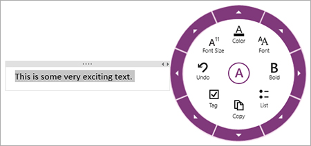
Dropdown menus are the more user-friendly option. Even though they technically take longer to select an option — users have to do a longer cursor movement to find their buttons — drop-down menus are more visually pleasing and hog less space than pie menus. They also unclutter your interface and organize its content into hierarchies and different groups. This allows you to have multiple dropdown menus right next to each other with submenus in all of them, without having to sacrifice the aesthetic of your page or a ton of whitespace, like HubSpot’s homepage below.

Fitts’s law also suggests that you should decrease the distance between objects that users use in a logical order. For instance, the login button is always right next to the username and password form fields.
When certain buttons are related, you should organize them in a way that’s easy to remember and find. Grouping similar buttons creates a familiar mental map on your website that users can basically memorize.
But placing every comparable button right next to each other could clutter your page and lead to a lot of user mistakes, especially if you put a high risk button, like a delete email button, right next to a frequently used button, like a send email button. To reduce these accidental actions, there should either be a two-step method to verify the action, an undo option, or ample space between the buttons.
3. Effort | Google and Apple
A lot of vital commands like ‘exit’, ‘start’, and ‘shut down’ are located in the corners of your computer screen. Placing buttons there makes it easier for users to select them because the buttons are pinned by two sides. And the cursor stops at each side, so you can’t go beyond them. This means you don’t have be as precise when you want to click a button in a corner or edge. You just have to move your cursor to its general vicinity.
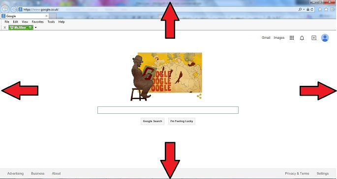
Placing buttons in corners and edges isn’t as user friendly on mobile devices, though. If you place them there, users need to stretch their fingers or move their hands just to reach them.
Less effort isn’t always better either. Crucial commands that are easy to do like turning off your phone doesn’t allow users to minimize the costs of their mistakes. Once they trigger them, users can’t undo them. There’s no forgiveness in the design at all.
To prevent frequent accidental shutdowns on their phones, Apple makes users swipe a slider to turn off their phone. And to rescind a power off, all users have to do is press the cancel button. The cancel button’s consequence doesn’t compare to turning the phone off, so Apple makes it easier to accidentally press it.

Fitts’s law is incredibly useful, but it isn’t full proof. Data always trumps theory, especially when testing user experience, so consider tracking the way users use your website and optimize its design for usability and conversions. Remember, Fitts’s law should never be a hard rule in user experience design. But it should always be an essential guideline.

24 Excel Formulas, Keyboard Shortcuts & Tricks That’ll Save You Lots of Time
Marketing and Microsoft Excel go together like peanut butter and chocolate. There’s just one problem.
For many of us, trying to organize and analyze Excel worksheets can feel like walking into a brick wall over and over again. You’re manually replicating columns and scribbling down long-form math on a scrap of paper, all while thinking to yourself, “There has to be a better way to do this.”
Truth be told, there is — you just don’t know it yet.
Excel can be tricky that way. On one hand, it’s an exceptionally powerful tool for reporting and analyzing marketing data. On the other, without the proper training, it’s easy to feel like it’s working against you. For starters, there are more than a dozen critical formulas Excel can automatically run for you so you’re not combing through hundreds of cells with a calculator on your desk.
Excel Formulas
- IF
- Percentage
- Subtraction
- Multiplication
- Division
- DATE
- Array
- COUNT
- AVERAGE
- SUMIF
- TRIM
- LEFT, MID, and RIGHT
- VLOOKUP
- RANDOMIZE
To help you use Excel more effectively (and save a ton of time), we’ve compiled a list of essential formulas, keyboard shortcuts, and other small tricks and functions you should know.
NOTE: The following formulas apply to Excel 2017. If you’re using a slightly older version of Excel, the location of each feature mentioned below might be slightly different.
IF Formula in Excel
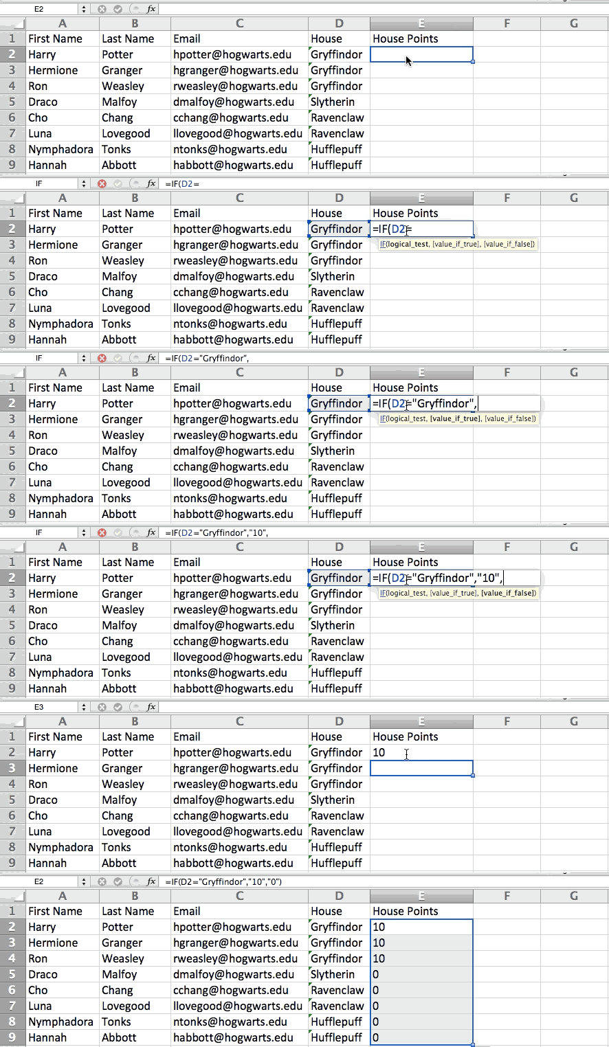
The IF formula in Excel is denoted =IF(logical_test, value_if_true, value_if_false). This allows you to enter a text value into the cell “if” something else in your spreadsheet is true or false. For example, =IF(D2=”Gryffindor”,”10″,”0″) would award 10 points to cell D2 if that cell contained the word “Gryffindor.”
There are times when we want to know how many times a value appears in our spreadsheets. But there are also those times when we want to find the cells that contain those values, and input specific data next to it.
We’ll go back to Sprung’s example for this one. If we want to award 10 points to everyone who belongs in the Gryffindor house, instead of manually typing in 10’s next to each Gryffindor student’s name, we’ll use the IF-THEN formula to say: If the student is in Gryffindor, then he or she should get ten points.
- The formula: IF(logical_test, value_if_true, value_if_false)
- Logical_Test: The logical test is the “IF” part of the statement. In this case, the logic is D2=”Gryffindor.” Make sure your Logical_Test value is in quotation marks.
- Value_if_True: If the value is true — that is, if the student lives in Gryffindor — this value is the one that we want to be displayed. In this case, we want it to be the number 10, to indicate that the student was awarded the 10 points. Note: Only use quotation marks if you want the result to be text instead of a number.
- Value_if_False: If the value is false — and the student does not live in Gryffindor — we want the cell to show “0,” for 0 points.
- Formula in below example: =IF(D2=”Gryffindor”,”10″,”0″)
Percentage Formula in Excel
To perform the percentage formula in Excel, enter the cells you’re finding a percentage for in the format, =A1/B1. To convert the resulting decimal value to a percentage, highlight the cell, click the Home tab, and select “Percentage” from the numbers dropdown.
There isn’t an Excel “formula” for percentages per se, but Excel makes it easy to convert the value of any cell into a percentage so you’re not stuck calculating and reentering the numbers yourself.
The basic setting to convert a cell’s value into a percentage is under Excel’s Home tab. Select this tab, highlight the cell(s) you’d like to convert to a percentage, and click into the dropdown menu next to Conditional Formatting (this menu button might say “General” at first). Then, select “Percentage” from the list of options that appears. This will convert the value of each cell you’ve highlighted into a percentage. See this feature below.
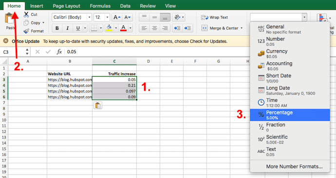
Keep in mind if you’re using other formulas, such as the division formula (denoted =A1/B1), to return new values, your values might show up as decimals by default. Simply highlight your cells before or after you perform this formula, and set these cells’ format to “Percentage” from the Home tab — as shown above.
Subtraction Formula in Excel
To perform the subtraction formula in Excel, enter the cells you’re subtracting in the format, =SUM(A1, -B1). This will subtract a cell using the SUM formula by adding a negative sign before the cell you’re subtracting. For example, if A1 was 10 and B1 was 6, =SUM(A1, -B1) would perform 10 + -6, returning a value of 4.
Like percentages, subtracting doesn’t have its own formula in Excel either, but that doesn’t mean it can’t be done. You can subtract any values (or those values inside cells) two different ways.
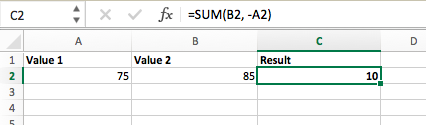
- Using the =SUM formula. To subtract multiple values from one another, enter the cells you’d like to subtract in the format =SUM(A1, -B1), with a negative sign (denoted with a hyphen) before the cell whose value you’re subtracting. Press enter to return the difference between both cells included in the parentheses. See how this looks in the screenshot above.
- Using the format, =A1-B1. To subtract multiple values from one another, simply type an equals sign followed by your first value or cell, a hyphen, and the value or cell you’re subtracting. Press Enter to return the difference between both values.
Multiplication Formula in Excel
To perform the multiplication formula in Excel, enter the cells you’re multiplying in the format, =A1*B1. This formula uses an asterisk to multiply cell A1 by cell B1. For example, if A1 was 10 and B1 was 6, =A1*B1 would return a value of 60.
You might think multiplying values in Excel has its own formula or uses the “x” character to denote multiplication between multiple values. Actually, it’s as easy as an asterisk — *.
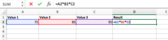
To multiply two or more values in an Excel spreadsheet, highlight an empty cell. Then, enter the values or cells you want to multiply together in the format, =A1*B1*C1 … etc. The asterisk will effectively multiply each value included in the formula.
Press Enter to return your desired product. See how this looks in the screenshot above.
Excel Division Formula
To perform the division formula in Excel, enter the cells you’re dividing in the format, =A1/B1. This formula uses a forward slash, “/,” to divide cell A1 by cell B1. For example, if A1 was 5 and B1 was 10, =A1/B1 would return a decimal value of 0.5.
Division in Excel is one of the simplest functions you can perform. To do so, highlight an empty cell, enter an equals sign, “=,” and follow it up with the two (or more) values you’d like to divide with a forward slash, “/,” in between. The result should be in the following format: =B2/A2, as shown in the screenshot below.
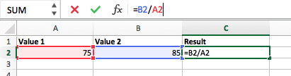
Hit Enter, and your desired quotient should appear in the cell you initially highlighted.
Excel DATE Formula
The Excel DATE formula is denoted =DATE(year, month, day). This formula will return a date that corresponds to the values entered in the parentheses — even values referred from other cells. For example, if A1 was 2018, B1 was 7, and C1 was 11, =DATE(A1,B1,C1) would return 7/11/2018.
Creating dates in the cells of an Excel spreadsheet can be a fickle task every now and then. Luckily, there’s a handy formula to make formatting your dates easy. There are two ways to use this formula:
- Create dates from a series of cell values. To do this, highlight an empty cell, enter “=DATE,” and in parentheses, enter the cells whose values create your desired date — starting with the year, then the month number, then the day. The final format should look like this: =DATE(year, month, day). See how this looks in the screenshot below.
- Automatically set today’s date. To do this, highlight an empty cell and enter the following string of text: =DATE(YEAR(TODAY()), MONTH(TODAY()), DAY(TODAY())). Pressing enter will return the current date you’re working in your Excel spreadsheet.
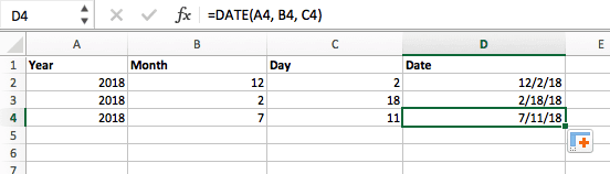
In either usage of Excel’s date formula, your returned date should be in the form of “mm/dd/yy” — unless your Excel program is formatted differently.
Excel Array Formula
An array formula in Excel surrounds a simple formula in brace characters using the format, {=(Start Value 1:End Value 1)*(Start Value 2:End Value 2)}. By pressing ctrl+shift+center, this will calculate and return value from multiple ranges, rather than just individual cells added to or multiplied by one another.
Calculating the sum, product, or quotient of individual cells is easy — just use the =SUM formula and enter the cells, values, or range of cells you want to perform that arithmetic on. But what about multiple ranges? How do you find the combined value of a large group of cells?
Numerical arrays are a useful way to perform more than one formula at the same time in a single cell so you can see one final sum, difference, product, or quotient. If you’re looking to find total sales revenue from several sold units, for example, the array formula in Excel is perfect for you. Here’s how you’d do it:
- To start using the array formula, type “=SUM,” and in parentheses, enter the first of two (or three, or four) ranges of cells you’d like to multiply together. Here’s what your progress might look like: =SUM(C2:C5
- Next, add an asterisk after the last cell of the first range you included in your formula. This stands for multiplication. Following this asterisk, enter your second range of cells. You’ll be multiplying this second range of cells by the first. Your progress in this formula should now look like this: =SUM(C2:C5*D2:D5)
- Ready to press Enter? Not so fast … Because this formula is so complicated, Excel reserves a different keyboard command for arrays. Once you’ve closed the parentheses on your array formula, press Ctrl+Shift+Enter. This will recognize your formula as an array, wrapping your formula in brace characters and successfully returning your product of both ranges combined.
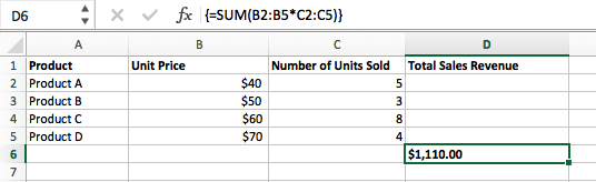
In revenue calculations, this can cut down on your time and effort significantly. See the final formula in the screenshot below.
COUNT Formula in Excel
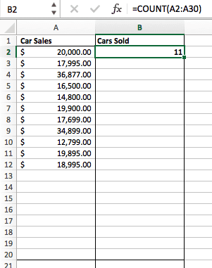
The COUNT formula in Excel is denoted =COUNT(Start Cell:End Cell). This formula will return a value that is equal to the number of entries found within your desired range of cells. For example, if there are eight cells with entered values between A1 and A10, =COUNT(A1:A10) will return a value of 8.
The COUNT formula in Excel is particularly useful for large spreadsheets, wherein you want to see how many cells contain actual entries. Don’t be fooled: This formula won’t do any math on the values of the cells themselves. This formula is simply to find out how many cells in a selected range are occupied with something.
Using the formula in bold above, you can easily run a count of active cells in your spreadsheet. The result will look a little something like this:
AVERAGE Formula in Excel
To perform the average formula in Excel, enter the values, cells, or range of cells of which you’re calculating the average in the format, =AVERAGE(number1, number2, etc.) or =AVERAGE(Start Value:End Value). This will calculate the average of all the values or range of cells included in the parentheses.
Finding the average of a range of cells in Excel keeps you from having to find individual sums and then performing a separate division equation on your total. Using =AVERAGE as your initial text entry, you can let Excel do all the work for you.
For reference, the average of a group of numbers is equal to the sum of those numbers, divided by the number of items in that group.
SUMIF Formula in Excel
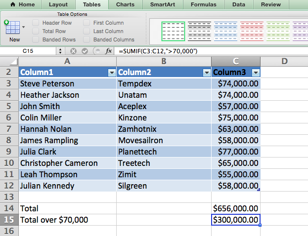
The SUMIF formula in Excel is denoted =SUMIF(range, criteria, [sum range]). This will return the sum of the values within a desired range of cells that all meet one criterion. For example, =SUMIF(C3:C12,”>70,000″) would return the sum of values between cells C3 and C12 from only the cells that are greater than 70,000.
Let’s say you want to determine the profit you generated from a list of leads who are associated with specific area codes, or calculate the sum of certain employees’ salaries — but only if they fall above a particular amount. Doing that manually sounds a bit time-consuming, to say the least.
With the SUMIF function, it doesn’t have to be — you can easily add up the sum of cells that meet certain criteria, like in the salary example above.
- The formula: =SUMIF(range, criteria, [sum_range])
- Range: The range that is being tested using your criteria.
- Criteria: The criteria that determine which cells in Criteria_range1 will be added together
- [Sum_range]: An optional range of cells you’re going to add up in addition to the first Range entered. This field may be omitted.
In the example below, we wanted to calculate the sum of the salaries that were greater than $70,000. The SUMIF function added up the dollar amounts that exceeded that number in the cells C3 through C12, with the formula =SUMIF(C3:C12,”>70,000″).
TRIM Formula in Excel
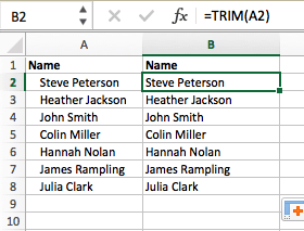
The TRIM formula in Excel is denoted =TRIM(text). This formula will remove any spaces entered before and after the text entered in the cell. For example, if A2 includes the name ” Steve Peterson” with unwanted spaces before the first name, =TRIM(A2) would return “Steve Peterson” with no spaces in a new cell.
Email and file sharing are wonderful tools in today’s workplace. That is, until one of your colleagues sends you a worksheet with some really funky spacing. Not only can those rogue spaces make it difficult to search for data, but they also affect the results when you try to add up columns of numbers.
Rather than painstakingly removing and adding spaces as needed, you can clean up any irregular spacing using the TRIM function, which is used to remove extra spaces from data (except for single spaces between words).
- The formula: =TRIM(text).
- Text: The text or cell from which you want to remove spaces.
Here’s an example of how we used the TRIM function to remove extra spaces before a list of names. To do so, we entered =TRIM(“A2”) into the Formula Bar, and replicated this for each name below it in a new column next to the column with unwanted spaces.
Below are some other Excel formulas you might find useful as your data management needs grow.
LEFT, MID, and RIGHT Formula
Let’s say you have a line of text within a cell that you want to break down into a few different segments. Rather than manually retyping each piece of the code into its respective column, users can leverage a series of string functions to deconstruct the sequence as needed: LEFT, MID, or RIGHT.
LEFT:
- Purpose: Used to extract the first X numbers or characters in a cell.
- The formula: =LEFT(text, number_of_characters)
- Text: The string that you wish to extract from.
- Number_of_characters: The number of characters that you wish to extract starting from the left-most character.
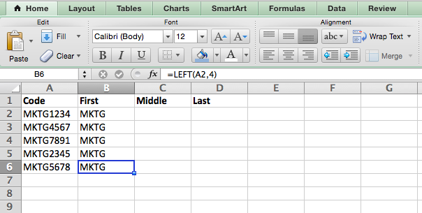
In the example below, we entered =LEFT(A2,4) into cell B2, and copied it into B3:B6. That allowed us to extract the first 4 characters of the code.
MID:
- Purpose: Used to extract characters or numbers in the middle based on position.
- The formula: =MID(text, start_position, number_of_characters)
- Text: The string that you wish to extract from.
- Start_position: The position in the string that you want to begin extracting from. For example, the first position in the string is 1.
- Number_of_characters: The number of characters that you wish to extract.
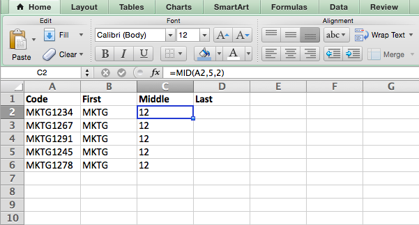
In this example, we entered =MID(A2,5,2) into cell B2, and copied it into B3:B6. That allowed us to extract the two numbers starting in the fifth position of the code.
RIGHT:
- Purpose: Used to extract the last X numbers or characters in a cell.
- The formula: =RIGHT(text, number_of_characters)
- Text: The string that you wish to extract from.
- Number_of_characters: The number of characters that you want to extract starting from the right-most character.
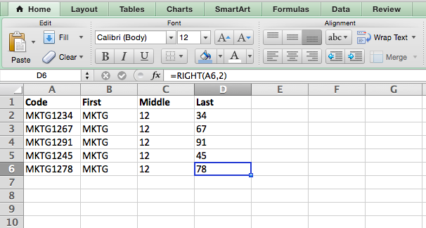
For the sake of this example, we entered =RIGHT(A2,2) into cell B2, and copied it into B3:B6. That allowed us to extract the last two numbers of the code.
VLOOKUP Formula
This one is an oldie, but a goodie — and it’s a bit more in depth than some of the other formulas we’ve listed here. But it’s especially helpful for those times when you have two sets of data on two different spreadsheets, and want to combine them into a single spreadsheet.
My colleague, Rachel Sprung — whose “How to Use Excel” tutorial is a must-read for anyone who wants to learn — uses a list of names, email addresses, and companies as an example. If you have a list of people’s names next to their email addresses in one spreadsheet, and a list of those same people’s email addresses next to their company names in the other, but you want the names, email addresses, and company names of those people to appear in one place — that’s where VLOOKUP comes in.
Note: When using this formula, you must be certain that at least one column appears identically in both spreadsheets. Scour your data sets to make sure the column of data you’re using to combine your information is exactly the same, including no extra spaces.
- The formula: VLOOKUP(lookup value, table array, column number, [range lookup])
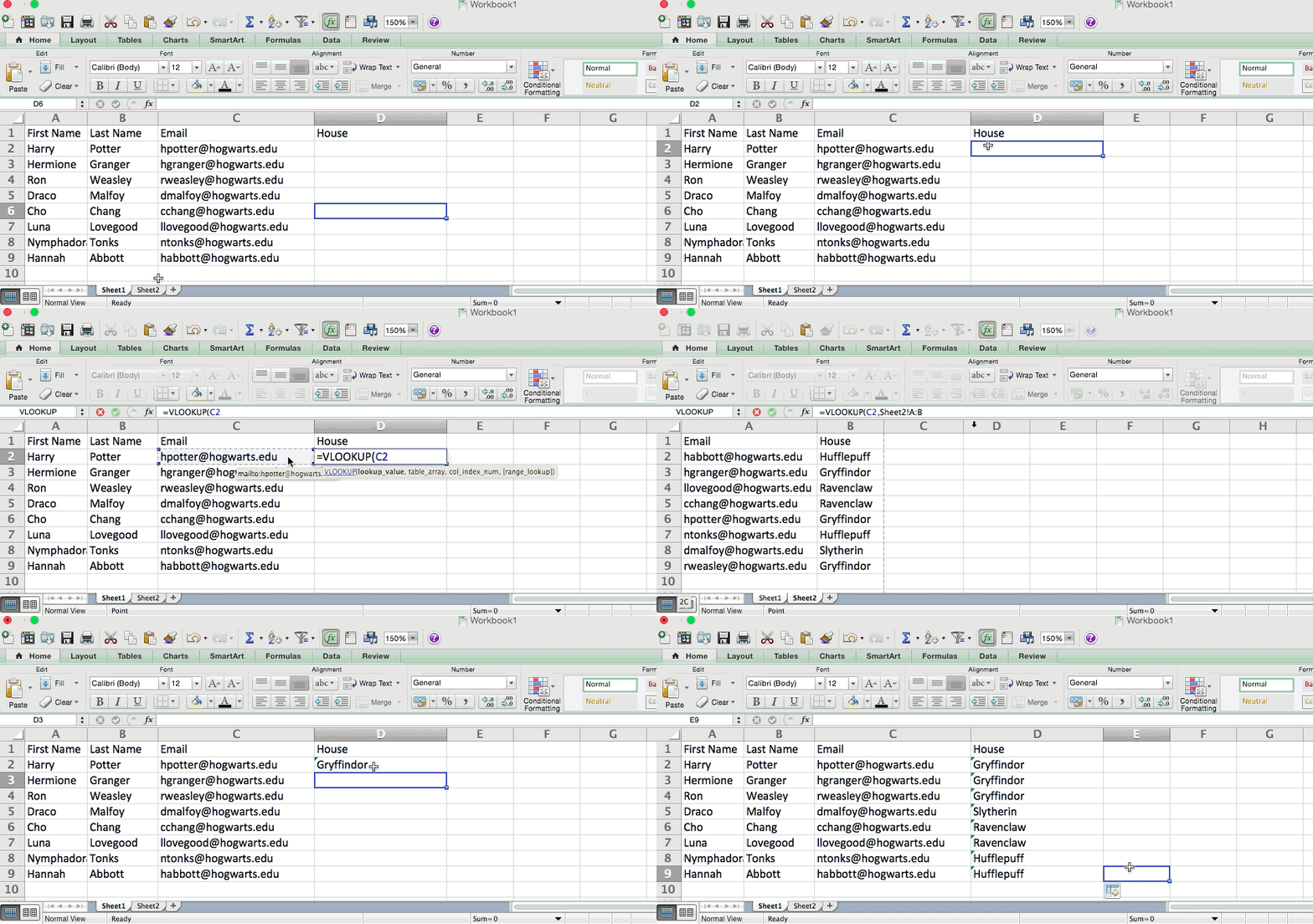
- Lookup Value: The identical value you have in both spreadsheets. Choose the first value in your first spreadsheet. In Sprung’s example that follows, this means the first email address on the list, or cell 2 (C2).
- Table Array: The range of columns on Sheet 2 you’re going to pull your data from, including the column of data identical to your lookup value (in our example, email addresses) in Sheet 1 as well as the column of data you’re trying to copy to Sheet 1. In our example, this is “Sheet2!A:B.” “A” means Column A in Sheet 2, which is the column in Sheet 2 where the data identical to our lookup value (email) in Sheet 1 is listed. The “B” means Column B, which contains the information that’s only available in Sheet 2 that you want to translate to Sheet 1.
- Column Number: The table array tells Excel where (which column) the new data you want to copy to Sheet 1 is located. In our example, this would be the “House” column, the second one in our table array, making it column number 2.
- Range Lookup: Use FALSE to ensure you pull in only exact value matches.
- The formula with variables from Sprung’s example below: =VLOOKUP(C2,Sheet2!A:B,2,FALSE)
In this example, Sheet 1 and Sheet 2 contain lists describing different information about the same people, and the common thread between the two is their email addresses. Let’s say we want to combine both datasets so that all the house information from Sheet 2 translates over to Sheet 1. Here’s how that would work:
RANDOMIZE Formula
There’s a great article that likens Excel’s RANDOMIZE formula to shuffling a deck of cards. The entire deck is a column, and each card — 52 in a deck — is a row. “To shuffle the deck,” writes Steve McDonnell, “you can compute a new column of data, populate each cell in the column with a random number, and sort the workbook based on the random number field.”
In marketing, you might use this feature when you want to assign a random number to a list of contacts — like if you wanted to experiment with a new email campaign and had to use blind criteria to select who would receive it. By assigning numbers to said contacts, you could apply the rule, “Any contact with a figure of 6 or above will be added to the new campaign.”
- The formula: RAND()
- Start with a single column of contacts. Then, in the column adjacent to it, type “RAND()” — without the quotation marks — starting with the top contact’s row.
- For the example below: RANDBETWEEN(bottom,top)
- RANDBETWEEN allows you to dictate the range of numbers that you want to be assigned. In the case of this example, I wanted to use one through 10.
- bottom: The lowest number in the range.
- top: The highest number in the range,
- Formula in below example: =RANDBETWEEN(1,10)
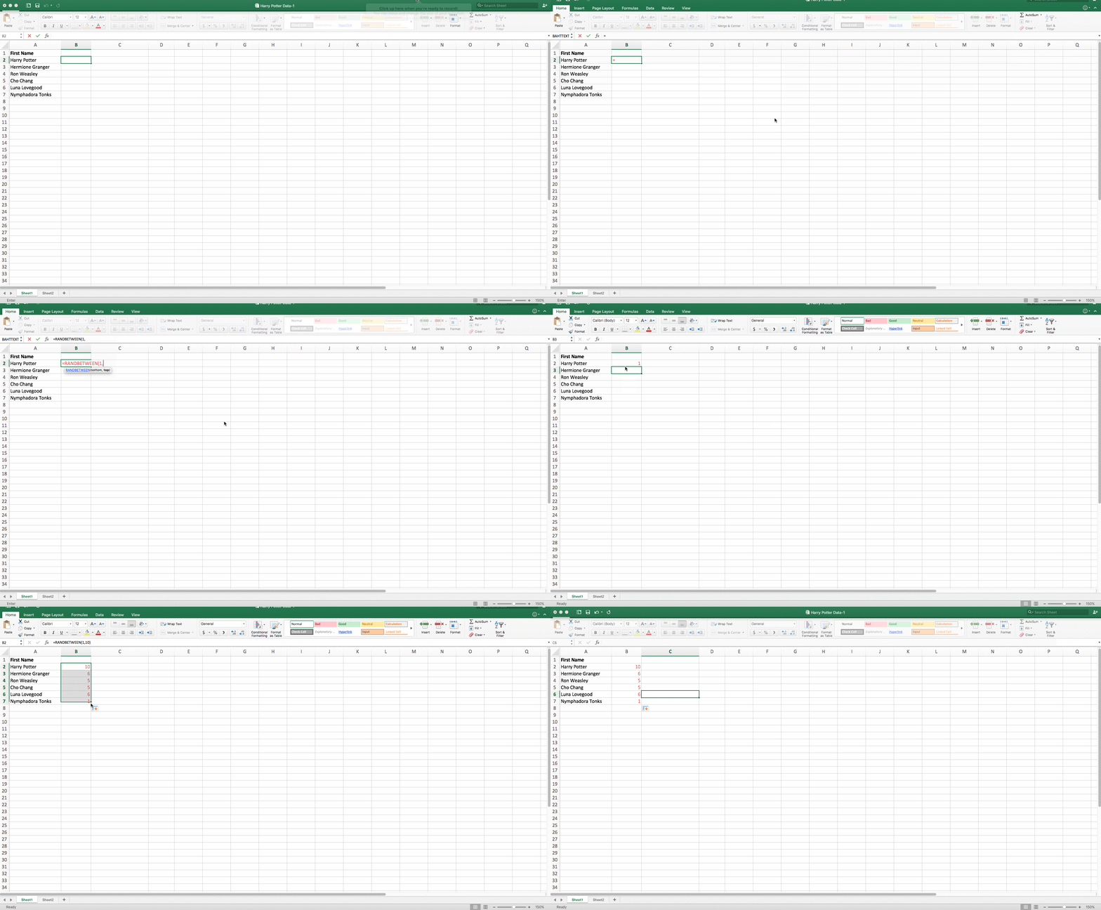
Helpful stuff, right? Now for the icing on the cake: Once you’ve mastered the Excel formula you need, you’ll want to replicate it for other cells without rewriting the formula. And luckily, there’s an Excel function for that, too. Check it out below.
How to Copy Formula in Excel
- Type your formula into an empty cell.
- Press “Enter” to run the formula.
- Hover your cursor over the bottom-right corner of the cell containing the formula.
- Click and hold the small plus (“+”) sign that appears.
- Drag your cursor down the column.
- Release your mouse to copy the formula into each subsequent cell.
- Check each new value to ensure it corresponds to the correct cells.
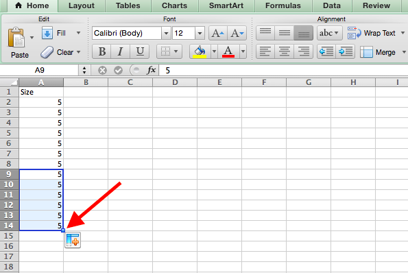
Tired of manually entering data that follows a pattern across a bunch of cells? Excel’s Auto Fill feature is designed to minimize the work required on your end, by making it easy to repeat values you’ve already input.
To do so, click and hold the lower right corner of a cell, and then drag it down or across into adjacent cells. When you release, Excel will fill in the adjacent cells with the data from the cell you first selected.
Excel Keyboard Shortcuts
Quickly select rows, columns, or the whole spreadsheet.
Perhaps you’re crunched for time. I mean, who isn’t? No time, no problem. You can select your entire spreadsheet in just one click. All you have to do is simply click the tab in the top-left corner of your sheet to highlight everything all at once.
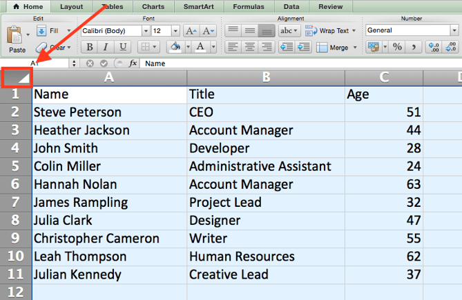
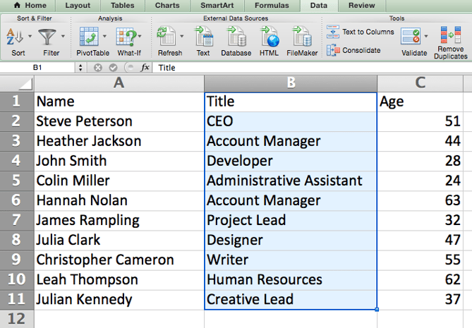
Just want to select everything in a particular column of row? That’s just as easy with these shortcuts:
For Mac:
- Select Column = Command + Shift + Down/Up
- Select Row = Command + Shift + Right/Left
For PC:
- Select Column = Control + Shift + Down/Up
- Select Row = Control + Shift + Right/Left
This shortcut is especially helpful when you’re working with larger data sets, but only need to select a specific piece of it.
Quickly open, close, or create a workbook.
Need to open, close, or create a workbook on the fly? The following keyboard shortcuts will enable you to complete any of the above actions in less than a minute’s time.
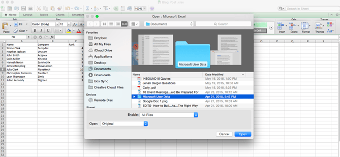
For Mac:
- Open = Command + O
- Close = Command + W
- Create New = Command + N
For PC:
- Open = Control + O
- Close = Control + F4
- Create New = Control + N
Format numbers into currency.
Have raw data that you want to turn into currency? Whether it be salary figures, marketing budgets, or ticket sales for an event, the solution is simple. Just highlight the cells you wish to reformat, and select Control + Shift + $.
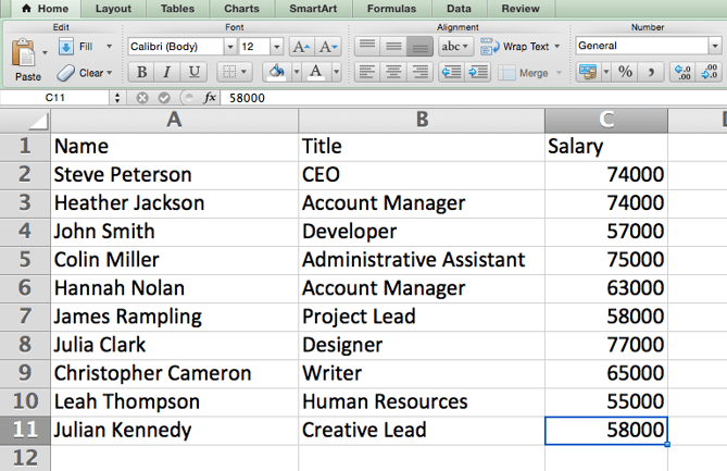
The numbers will automatically translate into dollar amounts — complete with dollar signs, commas, and decimal points.
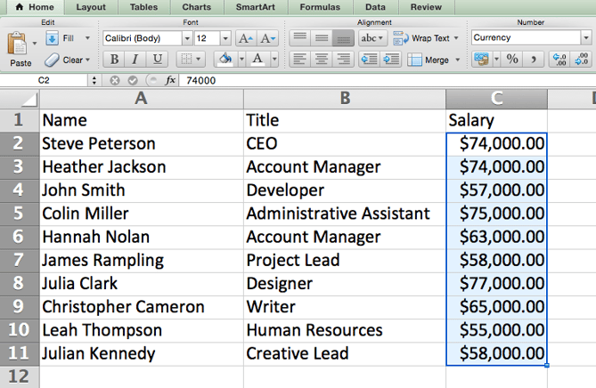
Note: This shortcut also works with percentages. If you want to label a column of numerical values as “percent” figures, replace “$” with “%”.
Insert current date and time into a cell.
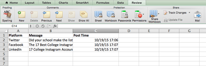
Whether you’re logging social media posts, or keeping track of tasks you’re checking off your to-do list, you might want to add a date and time stamp to your worksheet. Start by selecting the cell to which you want to add this information.
Then, depending on what you want to insert, do one of the following:
- Insert current date = Control + ; (semi-colon)
- Insert current time = Control + Shift + ; (semi-colon)
- Insert current date and time = Control + ; (semi-colon), SPACE, and then Control + Shift + ; (semi-colon).
Other Excel Tricks
Customize the color of your tabs.
If you’ve got a ton of different sheets in one workbook — which happens to the best of us — make it easier to identify where you need to go by color-coding the tabs. For example, you might label last month’s marketing reports with red, and this month’s with orange.
Simply right click a tab and select “Tab Color.” A popup will appear that allows you to choose a color from an existing theme, or customize one to meet your needs.
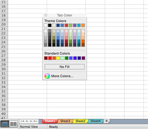
Add a comment to a cell.
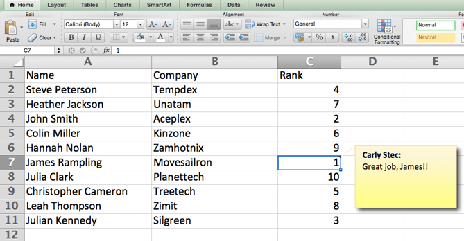
When you want to make a note or add a comment to a specific cell within a worksheet, simply right-click the cell you want to comment on, then click Insert Comment. Type your comment into the text box, and click outside the comment box to save it.
Cells that contain comments display a small, red triangle in the corner. To view the comment, hover over it.
Copy and duplicate formatting.
If you’ve ever spent some time formatting a sheet to your liking, you probably agree that it’s not exactly the most enjoyable activity. In fact, it’s pretty tedious.
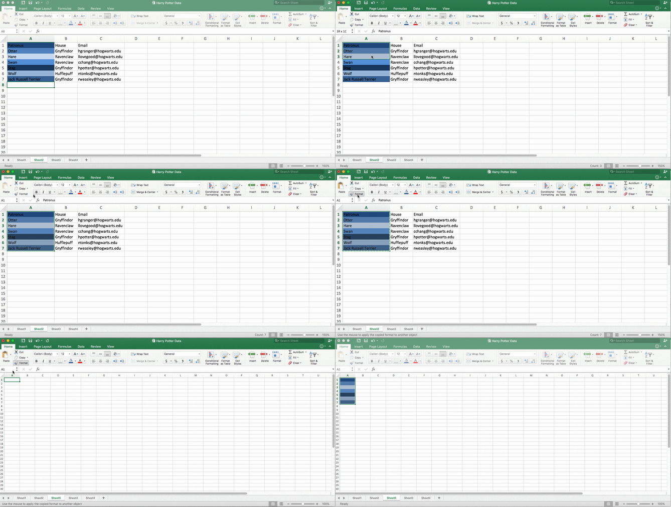
For that reason, it’s likely that you don’t want to repeat the process next time — nor do you have to. Thanks to Excel’s Format Painter, you can easily copy the formatting from one area of a worksheet to another.
Select what you’d like to replicate, then select the Format Painter option — the paintbrush icon — from the dashboard. The pointer will then display a paintbrush, prompting you to select the cell, text, or entire worksheet to which you want to apply that formatting, as shown below:
Identify duplicate values.
In many instances, duplicate values — like duplicate content when managing SEO — can be troublesome if gone uncorrected. In some cases, though, you simply need to be aware of it.
Whatever the situation may be, it’s easy to surface any existing duplicate values within your worksheet in just a few quick steps. To do so, click into the Conditional Formatting option, and select Highlight Cell Rules > Duplicate Values
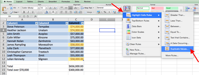
Using the popup, create the desired formatting rule to specify which type of duplicate content you wish to bring forward.
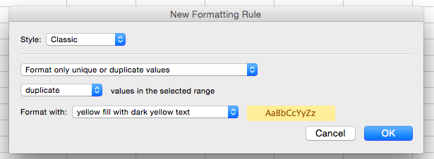
In the example above, we were looking to identify any duplicate salaries within the selected range, and formatted the duplicate cells in yellow.
In marketing, the use of Excel is pretty inevitable — but with these tricks, it doesn’t have to be so daunting. As they say, practice makes perfect. The more you use these formulas, shortcuts, and tricks, the more they’ll become second nature.
To dig a little deeper, check out a few of our favorite resources for learning Excel. Want more Excel tips? Check out this post on how to create a pivot table with medians.



macOS: How to enable Dock Magnification

One fun toggle that some users like to enable is the ability to enable Magnification on the Dock inside macOS. While this certainly isn’t a new feature, users may still want to know how to enable it.
Apple casts ‘Game of Thrones’ star Jason Momoa in upcoming ‘world-building drama’

Apple continues to ramp up its original content efforts today with a new show starring Jason Momoa. The show is entitled “See” and is said to be a “world-building drama” set in the future…
Apple could grow revenue by as much as $11 billion, analysts say

Apple has made it clear that augmented reality is a big area of focus as it moves forward, and analysts are beginning to agree. As noted by CNBC, Bank of America Merrill Lynch believes that AR could turn into an $8 billion revenue stream for Apple…
Former Apple employee faces up to 10 years in prison, $250K fine for stealing Project Titan trade secrets

The United States Federal Bureau of Investigation charged former Apple employee Xiaolang Zhang with stealing trade secrets. Zhang was hired back in December of 2015 by Apple to work on Project Titan, focusing mainly on software and hardware for autonomous vehicles.
How Apple dominated the World Cup despite not being an official sponsor

iPhone & iPad: How to get the official Apple user guides for free

Whether you’re new to iPhone or iPad, or just enjoy having the official user guides from Apple as a reference, having them on hand can be useful for yourself in addition to helping others.
9to5Mac Daily: July 10, 2018

Listen to a recap of the top stories of the day from 9to5Mac. 9to5Mac Daily is available on iTunes and Apple’s Podcasts app, Stitcher, TuneIn, Google Play, or through our dedicated RSS feed for Overcast and other podcast players.
What You Missed at Google’s Marketing Innovations Keynote
Last month, Google let the world know that big changes were coming to its famed AdWords.
Those changes would come in the form of a major rebrand — and what was once AdWords is now a suite of three separate brands: Google Ads, Google Marketing Platform, and Google Ad Manager.
Today, all three took center stage at Google Marketing Live, where the Marketing Innovations keynote went into a bit more detail about these changes — and the purpose they ultimately serve for those who use them.
But it was almost as if today’s key takeaways had more to do with reverberating themes echoed throughout the keynote than the products themselves — things that Google, for some time now, has worked to make synonymous with its name and its brand. Things like machine learning, personalization, and solving for user experience.
Here’s a closer look at some of them.
What You Missed at Google’s Marketing Innovations Keynote
Google Puts Machine Learning Center Stage
Machine learning is what many think of as Google’s “thing.” It plays a major part in what shapes the search algorithm, as well as in the latest updates to Gmail (e.g., smart compose), and it helped to build the controversial Google Duplex: technology that allows Google Assistant to make strikingly human-like calls to make appointments and reservations.
Ads are no exception to Google’s machine learning initiatives. But that’s not new to today’s announcements, as the company announced “Smart display campaigns,” for example, over a year ago.
Still, machine learning is informing the latest generation of Google’s ad- and marketing-focused offerings — and is lending itself, says SVP of Ads and Commerce Sridhar Ramaswamy, to the crucial nexus of assistance and personalization that makes a great ad.
“Ads should add value,” he told the audience.
Much of what was announced today takes on the responsibility of helping marketers figure out how to create such valuable ads. Take the concept of responsive search ads, for instance, where advertisers are asked to create a new ad with 15 possible headlines and four description lines.
From there, Google tests different combinations of both, using machine learning to determine which one has the greatest returns for a given search query.
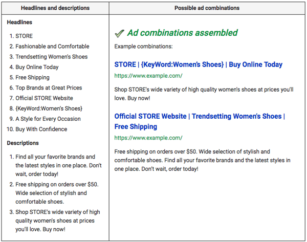
Source: Google
Goal-Oriented Campaigns
Not all ads are created equal.
That’s one reason why their ability to provide value is so crucial — not everyone is searching for the same thing.
That’s a phenomenon that Google has incorporated into its public “principles” of ads — and search, for that matter. And, it’s another place where machine learning comes in: to display the right ad for the right audience, allowing it to provide both the assistance and personalization Ramaswamy alluded to.
But advertisers — and the businesses behind them — all have different intended outcomes, too, that go beyond the bottom line. For brick-and-mortar retailers, for instance, bringing customers through the front door might be a key goal (which Google also said it will address with its new local campaign tools).
Google today introduced a way to customize various types of campaigns — Search, Display, Shopping, or Video — specifically around an advertiser’s goals.
Machine learning isn’t quite as front-and-center here, but likely has informed the recommendations that Google makes to advertisers when they input these goals — based on what it’s learned historically about consumer behavior.
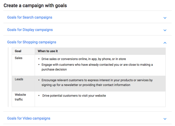
Source: Google
The Merging of Analytics and Advertising
As valuable as these new tools and the technology behind them might be, it’s equally important to measure the return on any investment made in them.
That’s why there’s often an emphasis on metrics. The ability to determine what caused a customer convert — like a specific ad, for instance — as well as how and why is especially important when something like a funded ad or campaign is concerned.
It also makes sense to be able to have all of that information in one place. And instead of keeping analytics and campaign content in separate silos, Google has introduced Display & Video 360 to synthesizes what used to be such fragmented ad products — such as DoubleClick Bid Manager, Campaign Manager, and Audience Center — into a single product.

Source: Google
Looking Ahead
What really underscored today’s announcements is the ability to address and adapt to the rapid evolution of consumer preferences and behavior — and to know if efforts to do so are working.
Marketers and advertisers are faced with the challenge of achieving an ideal promotional trifecta — of what Google Ads Group Product Manager Philip McDonnell identified as the right product, in front of the right person, at the right time.
That works in tandem with the technology people use to seek information, which Ramaswamy was keen to point out “has been changing at an unrelenting pace.”
It’s why HubSpot Head of SEO Victor Pan, who previously managed multi-million-dollar digital advertising strategies, advises marketers to be patient.
“Google will likely train and retrain its machine learning — based on input from the early adapters among advertisers who work with these tools,” he says. “The technology will only continue to evolve.”
But ultimately, marketers — including those within small-to-midsize businesses — should be able to adapt.
“Google’s trying to demystify machine learning to a larger audience through adoption,” Pan explains. “What better way to do that via Google Ads?”
The full rebrand of Google AdWords into Google Ads is scheduled to take place on July 24th. We’ll be monitoring these changes as they launch, and providing updates on if/how these changes will be reflected within HubSpot.
Featured image source: Google

Apple groups Siri and Machine Learning teams, ex-Google hire Giannandrea named Chief of ML and AI

As Apple hired away Google’s chief of search and AI this past spring, Tim Cook noted that he would be heading up the company’s AI and machine learning strategy. Now, we’re hearing news about how some teams are being restructured that could bring future improvements to Siri and more.
Instagram Stories getting more interactive with new ‘Question Sticker’ conversation starters

9to5Toys Lunch Break: Beats Solo3 Headphones $160, GoPro HERO6 $329, Belkin USB-C Express Dock $80, more

Keep up with the best gear and deals on the web by signing up for the 9to5Toys Newsletter. Also, be sure to check us out on: Twitter, RSS Feed, Facebook, Google+ and Safari push notifications.
Listen to the new 9to5Toys Daily Podcast:
Apple Maps is being rebooted, but Google Maps has a huge adoption lead

A new report out today on navigation app trends sheds some light on how far Google Maps could be ahead of Apple Maps and other services. Included are the top reasons why almost 70% of users are sticking with Google Maps.
AgileBits dismisses rumor Apple is buying 1Password

Is Apple buying 1Password? BGR thinks they might be, maybe! The source of this rumor is a headline from the site that includes “acquisition talks underway” in a story about Apple employees receiving 1Password memberships as a work perk.
I worked in Apple Retail in 2011 and had access to lots of similar perks so that alone doesn’t spell acquisition, but it is a nice benefit. The meat of the story is this bit: