Welcome to My Blog

When you’re selecting cover photos, shared images, and other social media assets, knowing the basic image dimensions might not cut it.

What if you want to make sure a certain part of your cover photo isn’t obstructed by your profile photo? And what’s the difference between shared link thumbnails, or in-stream photos — are the dimensions different for those?

As it turns out, sizing images correctly for social media is no simple task. Even just for Facebook marketing, photo dimensions vary according to where and how it’s shared — from cover photos, to timeline images, to profile pictures.

But if you’re looking for a detailed guide on social media image sizes, you’re in luck. See a written list of essential social media image dimensions below, sorted by social network and the type of image you’re posting.

 

Social Media Image Sizes

All image dimensions below are in pixels, width x height. To jump to a specific social network in this guide use the list below.

• Facebook Image Sizes
• Twitter Image Sizes
• Google+ Image Sizes
• Instagram Image Sizes
• Pinterest Images Sizes
• LinkedIn Image Sizes
• YouTube Image & Media Sizes
• Tumblr Image Sizes
• Snapchat Image Sizes

Facebook Image Sizes

Image Dimensions | File Sizes

• Cover image: 820 x 312 (minimum 400 x 150)
• Profile image: ≥180 x 180
• Shared post image: 1200 x 630
• Shared link preview image: 1200 x 628
• Event image: 1920 x 1080

With 1.5 billion daily active users, Facebook continues to outpace other social media channels. The images you use here are crucial — choosing a lower-quality one can make or break your engagement. Pro tip: The way images display on your own timeline might look different.

Your profile image will appear 170 x 170 on desktop, and 32 x 32 as a thumbnail associated with your Facebook posts.

Twitter Image Sizes

Image Dimensions | File Sizes

• Header image: 1500 x 500 | maximum 5 MB
• Profile image: 400 x 400 | maximum 2 MB
• In-stream image: 440 x 220

Twitter, meanwhile, is often the social network of choice for users to talk about you. It’s where customers ask questions, leave praise, and request help. But, the format and display have changed several times in the course of its history, so here are the image dimensions you need to know.

Although your profile image will display 200 x 200 on most devices, you should still upload a photo that is 400 x 400.

Google+ Image Sizes

Update: Google recently announced it is shutting down its Google+ platform. Please consider using the dimensions below for any potential social networking platform Google launches in the future, and check back with us for an updated set of image dimensions that reflect this rollout.

Image Dimensions | File Sizes

• Profile image: 250 x 250 | maximum 100 MB
• Cover image: 1080 x 608 (minimum 480 x 270)
• Shared image: 497 x 373
• Shared video: ≥496 pixels wide
• Shared link image thumbnail: 150 x 150

Google+ has historically been an important platform for small businesses who want to show up in local Google searches. This is true even if you think it might not get as much attention as other social media channels. The last thing you want is to have users stumble upon your profile there, only to find months (or more) of radio silence and distorted visual content.

Plus, where there’s Google+, there is Google, indicating a connection to the search giant itself.

Instagram Image Sizes

Image Dimensions | File Sizes

• Profile image: 110 x 110
• Image thumbnail: 161 x 161
• Shared photos: 1080 x 1080
• Shared videos: 1080 pixels wide
• Instagram Stories: 1080 x 1920 (minimum 600 x 1067) | maximum 4 GB

Given that Instagram’s bread-and-butter is visual content, you’ll want your presence on this channel to match that foundation, especially in terms of quality. And with more than 700 million daily active users, you’ll want to look your best.

Instagram scales shared photos down to 612 x 612. Nonetheless, you should still set these image posts to 1080 x 1080.

Pinterest Image Sizes

Image Dimensions | File Sizes

• Profile image: 165 x 165 | maximum 10 MB
• Board cover image: 222 x 150 (minimum 55 x 55)
• Pinned image preview: 236 pixels wide

Here’s a fun fact: 90% of content posted on Pinterest consists of external links. For that reason, it’s worthwhile to leverage Pinterest for referral traffic — but it still has to catch your audience’s eyes. Here are the dimensions to make sure your Pinterest presence maintains visual quality.

LinkedIn Image Sizes

Image Dimensions | File Sizes

• Banner image: 1584 x 396 | maximum 4 MB
• Profile image: 400 x 400 (minumum 200 x 200) | maximum 10 MB
• Company Cover image: 1536 x 768
• Shared image: 350 pixels wide
• Shared link preview: 180 x 110
• Company logo image: 300 x 300 | maximum 4 MB
• Company cover image: 1536 x 768 (minimum 1192 x 220) | maximum 4 MB
• Company page banner image: 646 x 220 | maximum 2 MB
• Square logo (appears in company searches): 60 x 60 | maximum 2 MB

Love it or hate it, LinkedIn is the social channel for digital professional networking. And depending on your industry, it can still be a good vehicle for traffic and discovery, especially within the B2B sector. Plus, if you’re using it for recruiting purposes, it’s important to present well on a job that several people use for research on job listings, as well as employer culture, location, and more.

YouTube Image & Media Sizes

Image Dimensions | File Sizes

• Channel cover images: 2560 x 1440 | maximum 4 MB
• Channel icon: 800 x 800
• Video thumbnail: 1280 x 720

Here’s another network where visual content reigns supreme — not to mention, one with more than one billion users. Make sure your own visual assets match that underlying purpose and philosophy — not just with the videos you share on there, but with the profile presence you maintain.

Keep in mind that people use YouTube on many different types of devices, and your channel cover image will vary in appearance across each one. Images at 2560 x 1440 will be optimized for TV screens, while desktop computers will display them at 2560 x 423. Mobile devices will display YouTube cover art at 1546 x 423, while tablets will display them at 1855 x 423.

Tumblr Image Sizes

• Profile image: 128 x 128
• Image post: 500 x 750 (maximum 1280 x 1920) | maximum 10 MB

Tumblr has been called many things: a blogging platform, a social network, and a content-sharing center where marketers and consumers alike can, well, share whatever they want. And with 430 million blogs currently registered on the site, you’ve got company — so shape up and make sure your visuals fit the right dimensions.

Keep in mind that if you’re uploading animated GIFs, your image sizes and restrictions are a bit different than static photos. Specifically, animated GIFs must be less than 3 MB and no more than 540 pixels.

Snapchat Image Sizes

At long last, we arrive at Snapchat: yet another social media channel known primarily for its visual assets. When it comes to using this network for marketing purposes, dimensions are fairly uniform, whether you’re simply looking to use a geofilter, or you’re hoping to share an ad or sponsored lens.

• Geofilters, ads, and lenses: 1080 x 1920

Let’s say you hire a new marketing director, and a year later, you see a severe increase in turnover rates. Out of 15 employees, only seven from the prior year remain.

Undoubtedly, an increase in turnover rates can impact your team’s productivity and morale, and leave you nervous about the future of your department.

So how do you figure out what’s going wrong, or how your marketing director can improve her performance to ensure higher job satisfaction for her team?

To determine what causes employees to leave, and to create a better, happier employee experience moving forward, it’s critical you conduct productive exit interviews.

To ensure you’re asking the right questions during exit interviews and employing best practices to get optimal feedback from your employees, take a look at our Exit Interview Form template, followed by the best practices HubSpot’s HR Business Partner recommends.

Exit Interview Form Template

Once an employee has given her resignation letter, you’ll want to send her a form with some (or all) of the following questions. Give her time to submit her answers through the form before meeting with her to discuss her answers, face-to-face.

Here are some of the questions you’ll want your exit interview form to include:

1. How long have you been considering leaving our company?

2. How did the job match expectations?

3. What reason below primarily describes your reason for leaving?

a. New industry (significant career change)

b. Compensation

c. More opportunities for learning and growth

d. Personal Reasons

e. Manager/ Leadership quality

f. Day-to-day work environment/culture

4. If you have accepted a new position, please select all the items that are more attractive about your new role:

a. Better pay

b. Better culture

c. Better location/ commute

d. Different industry

e. Manager

f. Better work-life balance

g. More career advancement opportunities

5. What did you like most about your job?

6. What did you dislike about your job? What would you change about your job?

7. How would you describe the culture of our company?

8. How would you describe the general atmosphere in the office?

9. The quality of supervision is important to most people at work. How was your relationship with your manager?

10. What could your supervisor do to improve his or her management style and skill?

11. We try to be an employee-oriented company in which employees experience positive morale and motivation. What is your experience of employee morale and motivation in the company?

12. Please provide any context to further describe your reasons for leaving. Was there an event that led to this decision?

13. What were your reasons for joining our company originally? How have your feelings changed?

14. Do you believe your manager supported your professional development?

15. What are 1-2 things our company could do to promote a better workplace?

16. Please provide context and any additional feedback you’d like to provide on your manager.

Exit Interview Best Practices

According to a study conducted by The Society for Human Resource Management (SHRM), on average it costs a company between six to nine months of an employee’s salary to locate and train a replacement for them — so if the employee who’s leaving makes 60K, that can work out to anywhere between 30K and 45K in recruiting and training costs.

Undoubtedly, a high turnover rate can hurt your company financially. Additionally, a high turnover rate can lead to less productive teams, and lower employee morale overall.

Ultimately, an exit interview doesn’t just help you understand why your talent is leaving — it also helps you ensure you can implement strategies or cultural changes to improve the satisfaction of employees who stay.

However, it’s not always easy to discern what a highly productive exit interview looks like.

To learn more about exit interview best practices, I spoke with Winston Tuggle, an HR Business Partner at HubSpot.

When it comes to exit interview best practices, Tuggle suggests, “For conducting productive exit interviews, I think one key is asking the same questions of all people who leave. This structure allows us to codify the exit responses so we can extract actionable data around why people are leaving, and how we can improve the employee experience. We do this by having a standard exit interview form that leavers submit, and then have an unbiased third-party follow up in-person to go deeper on the answers the person filled out in the exit interview. Exit interviews aren’t necessary unless you plan on using them to gather as much data as possible that can be coupled with employee survey data to understand the employee experience.”

Tuggle also notes, “[It’s critical you understand] the ‘why’ behind someone leaving … to gather trends over time. As an HR team, it helps us to not overreact to one person’s experience and conversely helps us identify trends that we can proactively address before they lead to more unwanted attrition.”

Additionally, it’s important you explain the purpose behind the exit interview to each employee before you begin. You might say, “We hope to use your feedback to continuously improve our culture and business processes, so we are interested in your honest opinion on how your experience has been.”

You’ll also want to make sure your exit interviews are confidential between the HR team and employees. While data or general insights can be used to improve employee experience and should be shared with leadership, your employee needs to know her exact complaints won’t reach her old manager or coworkers.

Finally, be sure to thank your employee for taking the time to provide feedback during an exit interview. While one individual likely can’t pinpoint issues regarding an entire team or department, you’ll likely see commonalities over time that can help you determine how you can improve your workplace for the long-run.

Nowadays, marketers can measure almost everything, giving us an unprecedented ability to gauge the performance of our marketing campaigns.

But, sometimes, we can get overly obsessed with the metrics that look good on paper but don’t provide as much insight we think, like clicks and views. A high dose of traffic can prove your headline’s quality if you’re a blogger, but it doesn’t tell you the whole story of what path your visitors take on your blog, or how exactly they engage with the page.

Fortunately, there’s a data visualization tool that can show you which sections of your content generate the most engagement and which don’t. They’re called heat maps, and they can arm you with the data and insights needed to optimize your website copy, user experience, and conversion rate optimization to their fullest potential.

Below, we’ll go over the different types of heat maps you can use to measure your content’s ability to attract attention and the insights you can extract from each of them.

What Is a Heat Map?

A heat map is visual representation of the engagement a page on your website receives. It uses a color spectrum to determine which sections of your page are better at holding attention. The “hot” sections attract the most amount of attention, and the “cold” sections attract the least amount of attention.

The Different Types of Heat Maps and What They Can Tell You

There are three main types of heat maps: scroll maps, click maps, and hover maps.

Scroll maps show you the percentage of visitors who scroll through each section of your webpage. The hotter the section, the more visitors have viewed it. This data can help determine where you should place CTAs or important information on your webpage. Stark changes in color on your scroll map can also help determine which sections of your webpage lose visitors’ attention.

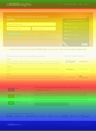
Image Credit: Impact

Click maps display the parts of your page that visitors click on the most. The hotter the section, the more frequently your visitors click on it. This data can show you if visitors care to click on your CTAs or other buttons that allow them to take a desired action. It can also show you if they’re getting distracted by non-clickable elements.

Image Credit: Hotjar

Hover maps show you where visitors hover their cursor while reading your webpage. The hotter the area, the longer they hang their cursor over it. This data can help determine how visitors actually navigate your website, so you can place important elements in a location where they’ll receive the greatest amount of attention possible. You can also figure out if non-essential elements are distracting your visitors from the important ones.

Image Credit: Pixeltr

Which Type of Content You Can Use Heat Maps On

Analyzing the heat map of each type of page on your website would be ideal, but, unfortunately, it isn’t efficient. The most effective way to leverage heat maps is to analyze the pages that influence your website’s conversion rate the most: your home page, landing pages, and high-conversion blog posts.

Home Page

Your homepage is an introduction to your brand. If you constantly monitor which sections visitors are scrolling through and whether they’re hovering over key information and clicking on CTAs, then you’ll know exactly where to place the most important elements of your homepage, reducing your bounce rate and increasing your conversion rate.

Landing Pages

Your landing pages are the last step in turning visitors into leads. If you can analyze your users’ behavior on these pages, then you can implement the optimal landing page design for generating the most amount of leads for your business.

High-Conversion Blog Posts

Your CTAs placement on your blog posts can heavily influence their conversion rate. For instance, at HubSpot, even though our end-of-post banner CTAs are visually engaging, we found out that they only generate a small fraction of our blog leads.

After analyzing our heat maps, we discovered that our anchor text CTAs, which are just hyperlinked blurbs of text located after each blog post’s introduction, actually generated the majority of our blog leads because most visitors saw the CTA at the beginning of the post and not the one at the end.

Prioritize Engagement, Not Vanity Metrics

Whether you’re A/B testing your website design or figuring out the best place to put a call-to-action on your blog posts, heat maps are your best tool for measuring attention and designing content that connects with your audience and converts them into leads and customers.

For most marketers, trying to organize and analyze spreadsheets in Microsoft Excel can feel like walking into a brick wall over and over again. You’re manually replicating columns and scribbling down long-form math on a scrap of paper, all while thinking to yourself, “There has to be a better way to do this.”

Truth be told, there is — you just don’t know it yet.

Excel can be tricky that way. On the one hand, it’s an exceptionally powerful tool for reporting and analyzing marketing data. On the other, without the proper training, it’s easy to feel like it’s working against you. For starters, there are more than a dozen critical formulas Excel can automatically run for you so you’re not combing through hundreds of cells with a calculator on your desk.

How to Insert Formulas in Excel

You might wonder what the “Formulas” tab on the top navigation toolbar in Excel means. In more recent versions of Excel, this horizontal menu — shown below — allows you to automatically find and insert Excel formulas into specific cells of your spreadsheet. 

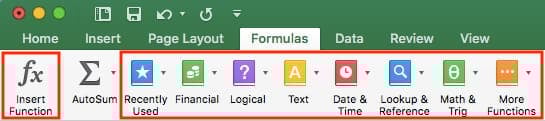
The more you use various formulas in Excel, the easier it’ll be to remember them and perform them manually. Nonetheless, the suite of icons above is a handy catalog of formulas you can browse and refer back to as you hone your spreadsheet skills.

Excel formulas are also called “functions.” To insert one into your spreadsheet, highlight a cell in which you want to run a formula, then click the far-left icon, “Insert Function,” to browse popular formulas and what they do. That browsing window will look like this:

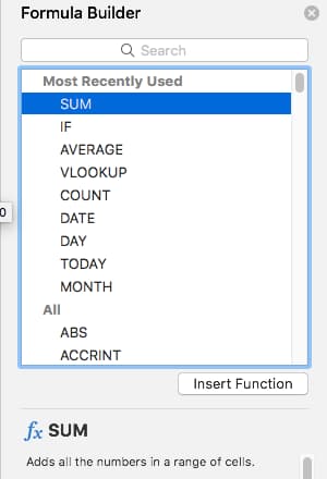Want a more sorted browsing experience? Use any of the icons we’ve highlighted (inside the long red rectangle in the first screenshot above) to find formulas related to a variety of common subjects — such as finance, logic, and more. Once you’ve found the formula that suits your needs, click “Insert Function,” as shown in the window above.

Now, let’s do a deeper dive into some of the most crucial Excel formulas and how to perform each one in typical situations.

To help you use Excel more effectively (and save a ton of time), we’ve compiled a list of essential formulas, keyboard shortcuts, and other small tricks and functions you should know.

NOTE: The following formulas apply to Excel 2017. If you’re using a slightly older version of Excel, the location of each feature mentioned below might be slightly different.

1. SUM  

All Excel formulas begin with the equals sign, =, followed by a specific text tag denoting the formula you’d like Excel to perform. 

The SUM formula in Excel is one of the most basic formulas you can enter into a spreadsheet, allowing you to find the sum (or total) of two or more values. To perform the SUM formula, enter the values you’d like to add together using the format, =SUM(value 1, value 2, etc).

The values you enter into the SUM formula can either be actual numbers or equal to the number in a specific cell of your spreadsheet. 

• To find the SUM of 30 and 80, for example, type the following formula into a cell of your spreadsheet: =SUM(30, 80). Press “Enter,” and the cell will produce the total of both numbers: 110. 
• To find the SUM of the values in cells B2 and B11, for example, type the following formula into a cell of your spreadsheet: =SUM(B2, B11). Press “Enter,” and the cell will produce the total of the numbers currently filled in cells B2 and B11. If there are no numbers in either cell, the formula will return 0. 

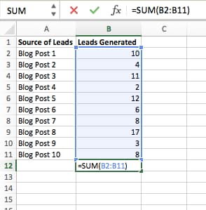
Keep in mind you can also find the total value of a list of numbers in Excel. To find the SUM of the values in cells B2 through B11, type the following formula into a cell of your spreadsheet: =SUM(B2:B11). Note the colon between both cells, rather than a comma. See how this might look in an Excel spreadsheet for a content marketer, below:

2. IF

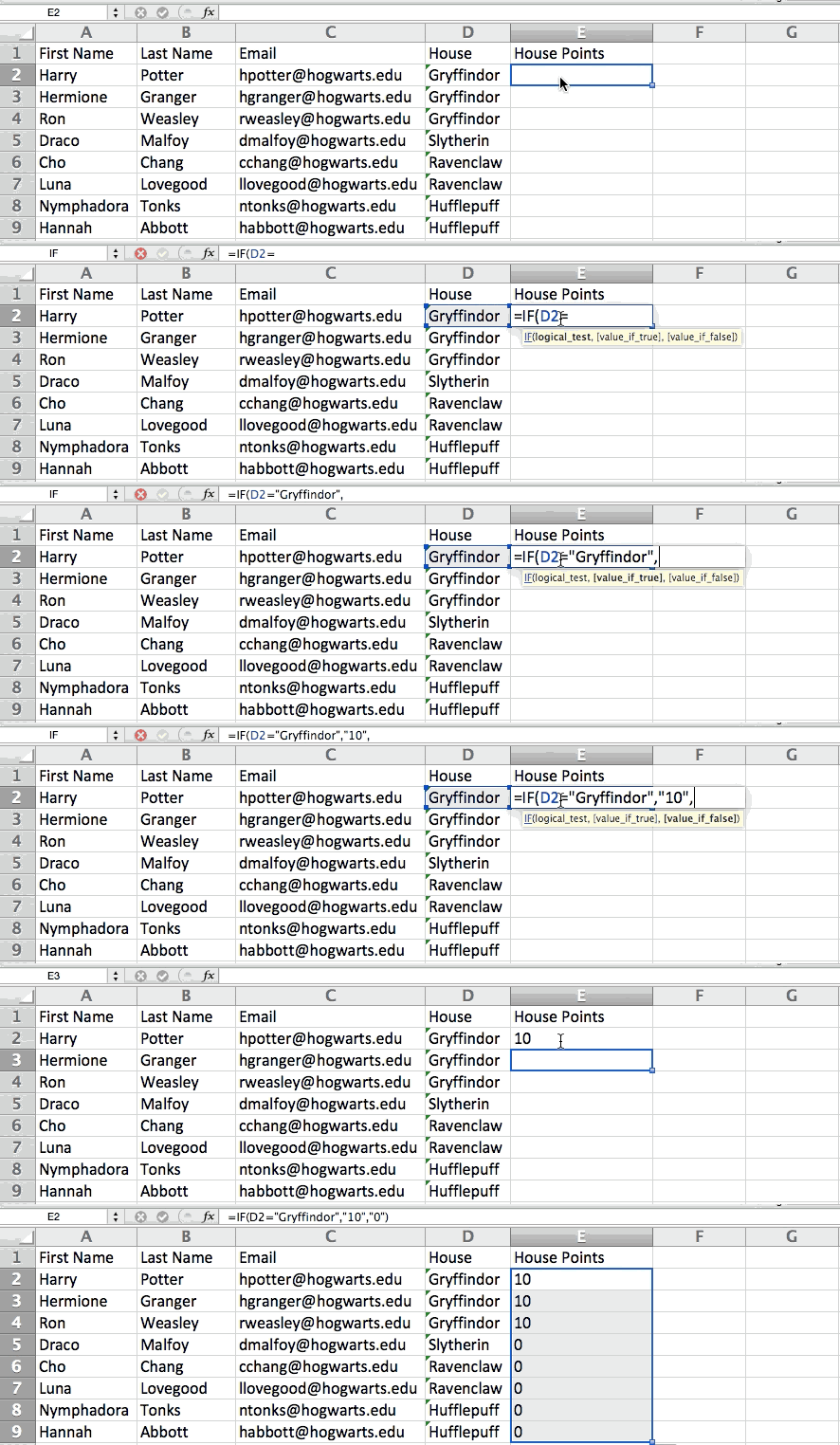
The IF formula in Excel is denoted =IF(logical_test, value_if_true, value_if_false). This allows you to enter a text value into the cell “if” something else in your spreadsheet is true or false. For example, =IF(D2=”Gryffindor”,”10″,”0″) would award 10 points to cell D2 if that cell contained the word “Gryffindor.”

There are times when we want to know how many times a value appears in our spreadsheets. But there are also those times when we want to find the cells that contain those values, and input specific data next to it.

We’ll go back to Sprung’s example for this one. If we want to award 10 points to everyone who belongs in the Gryffindor house, instead of manually typing in 10’s next to each Gryffindor student’s name, we’ll use the IF-THEN formula to say: If the student is in Gryffindor, then he or she should get ten points.

• The formula: IF(logical_test, value_if_true, value_if_false)
  • Logical_Test: The logical test is the “IF” part of the statement. In this case, the logic is D2=”Gryffindor.” Make sure your Logical_Test value is in quotation marks.
  • Value_if_True: If the value is true — that is, if the student lives in Gryffindor — this value is the one that we want to be displayed. In this case, we want it to be the number 10, to indicate that the student was awarded the 10 points. Note: Only use quotation marks if you want the result to be text instead of a number.
  • Value_if_False: If the value is false — and the student does not live in Gryffindor — we want the cell to show “0,” for 0 points.
• Formula in below example: =IF(D2=”Gryffindor”,”10″,”0″)

3. Percentage

To perform the percentage formula in Excel, enter the cells you’re finding a percentage for in the format, =A1/B1. To convert the resulting decimal value to a percentage, highlight the cell, click the Home tab, and select “Percentage” from the numbers dropdown.

There isn’t an Excel “formula” for percentages per se, but Excel makes it easy to convert the value of any cell into a percentage so you’re not stuck calculating and reentering the numbers yourself.

The basic setting to convert a cell’s value into a percentage is under Excel’s Home tab. Select this tab, highlight the cell(s) you’d like to convert to a percentage, and click into the dropdown menu next to Conditional Formatting (this menu button might say “General” at first). Then, select “Percentage” from the list of options that appears. This will convert the value of each cell you’ve highlighted into a percentage. See this feature below.

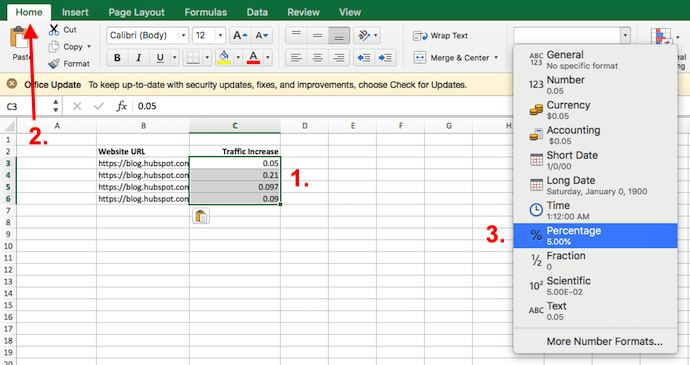
Keep in mind if you’re using other formulas, such as the division formula (denoted =A1/B1), to return new values, your values might show up as decimals by default. Simply highlight your cells before or after you perform this formula, and set these cells’ format to “Percentage” from the Home tab — as shown above.

4. Subtraction

To perform the subtraction formula in Excel, enter the cells you’re subtracting in the format, =SUM(A1, -B1). This will subtract a cell using the SUM formula by adding a negative sign before the cell you’re subtracting. For example, if A1 was 10 and B1 was 6, =SUM(A1, -B1) would perform 10 + -6, returning a value of 4.

Like percentages, subtracting doesn’t have its own formula in Excel either, but that doesn’t mean it can’t be done. You can subtract any values (or those values inside cells) two different ways.

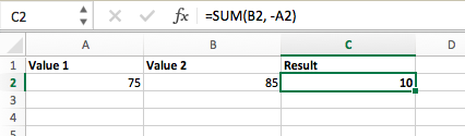
• Using the =SUM formula. To subtract multiple values from one another, enter the cells you’d like to subtract in the format =SUM(A1, -B1), with a negative sign (denoted with a hyphen) before the cell whose value you’re subtracting. Press enter to return the difference between both cells included in the parentheses. See how this looks in the screenshot above.
• Using the format, =A1-B1. To subtract multiple values from one another, simply type an equals sign followed by your first value or cell, a hyphen, and the value or cell you’re subtracting. Press Enter to return the difference between both values.

5. Multiplication

To perform the multiplication formula in Excel, enter the cells you’re multiplying in the format, =A1*B1. This formula uses an asterisk to multiply cell A1 by cell B1. For example, if A1 was 10 and B1 was 6, =A1*B1 would return a value of 60.

You might think multiplying values in Excel has its own formula or uses the “x” character to denote multiplication between multiple values. Actually, it’s as easy as an asterisk — *.

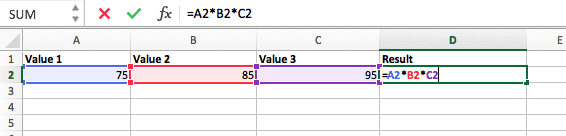
To multiply two or more values in an Excel spreadsheet, highlight an empty cell. Then, enter the values or cells you want to multiply together in the format, =A1*B1*C1 … etc. The asterisk will effectively multiply each value included in the formula.

Press Enter to return your desired product. See how this looks in the screenshot above.

6. Division

To perform the division formula in Excel, enter the cells you’re dividing in the format, =A1/B1. This formula uses a forward slash, “/,” to divide cell A1 by cell B1. For example, if A1 was 5 and B1 was 10, =A1/B1 would return a decimal value of 0.5.

Division in Excel is one of the simplest functions you can perform. To do so, highlight an empty cell, enter an equals sign, “=,” and follow it up with the two (or more) values you’d like to divide with a forward slash, “/,” in between. The result should be in the following format: =B2/A2, as shown in the screenshot below.

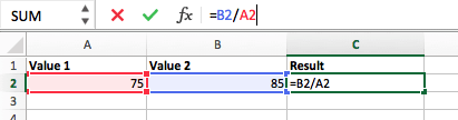
Hit Enter, and your desired quotient should appear in the cell you initially highlighted.

7. DATE

The Excel DATE formula is denoted =DATE(year, month, day). This formula will return a date that corresponds to the values entered in the parentheses — even values referred from other cells. For example, if A1 was 2018, B1 was 7, and C1 was 11, =DATE(A1,B1,C1) would return 7/11/2018.

Creating dates in the cells of an Excel spreadsheet can be a fickle task every now and then. Luckily, there’s a handy formula to make formatting your dates easy. There are two ways to use this formula:

• Create dates from a series of cell values. To do this, highlight an empty cell, enter “=DATE,” and in parentheses, enter the cells whose values create your desired date — starting with the year, then the month number, then the day. The final format should look like this: =DATE(year, month, day). See how this looks in the screenshot below.
• Automatically set today’s date. To do this, highlight an empty cell and enter the following string of text: =DATE(YEAR(TODAY()), MONTH(TODAY()), DAY(TODAY())). Pressing enter will return the current date you’re working in your Excel spreadsheet.

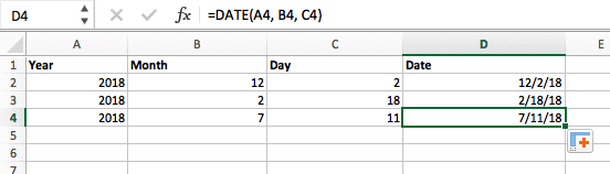
In either usage of Excel’s date formula, your returned date should be in the form of “mm/dd/yy” — unless your Excel program is formatted differently.

8. Array

An array formula in Excel surrounds a simple formula in brace characters using the format, {=(Start Value 1:End Value 1)*(Start Value 2:End Value 2)}. By pressing ctrl+shift+center, this will calculate and return value from multiple ranges, rather than just individual cells added to or multiplied by one another.

Calculating the sum, product, or quotient of individual cells is easy — just use the =SUM formula and enter the cells, values, or range of cells you want to perform that arithmetic on. But what about multiple ranges? How do you find the combined value of a large group of cells?

Numerical arrays are a useful way to perform more than one formula at the same time in a single cell so you can see one final sum, difference, product, or quotient. If you’re looking to find total sales revenue from several sold units, for example, the array formula in Excel is perfect for you. Here’s how you’d do it:

1. To start using the array formula, type “=SUM,” and in parentheses, enter the first of two (or three, or four) ranges of cells you’d like to multiply together. Here’s what your progress might look like: =SUM(C2:C5
2. Next, add an asterisk after the last cell of the first range you included in your formula. This stands for multiplication. Following this asterisk, enter your second range of cells. You’ll be multiplying this second range of cells by the first. Your progress in this formula should now look like this: =SUM(C2:C5*D2:D5)
3. Ready to press Enter? Not so fast … Because this formula is so complicated, Excel reserves a different keyboard command for arrays. Once you’ve closed the parentheses on your array formula, press Ctrl+Shift+Enter. This will recognize your formula as an array, wrapping your formula in brace characters and successfully returning your product of both ranges combined.

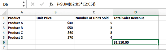
In revenue calculations, this can cut down on your time and effort significantly. See the final formula in the screenshot above.

9. COUNT

The COUNT formula in Excel is denoted =COUNT(Start Cell:End Cell). This formula will return a value that is equal to the number of entries found within your desired range of cells. For example, if there are eight cells with entered values between A1 and A10, =COUNT(A1:A10) will return a value of 8.

The COUNT formula in Excel is particularly useful for large spreadsheets, wherein you want to see how many cells contain actual entries. Don’t be fooled: This formula won’t do any math on the values of the cells themselves. This formula is simply to find out how many cells in a selected range are occupied with something.

Using the formula in bold above, you can easily run a count of active cells in your spreadsheet. The result will look a little something like this:

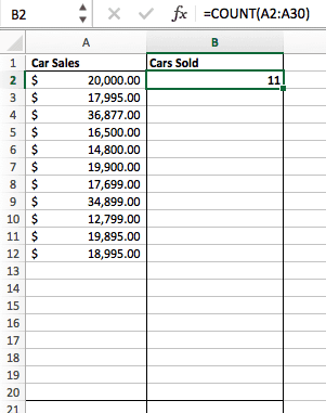
10. AVERAGE

To perform the average formula in Excel, enter the values, cells, or range of cells of which you’re calculating the average in the format, =AVERAGE(number1, number2, etc.) or =AVERAGE(Start Value:End Value). This will calculate the average of all the values or range of cells included in the parentheses.

Finding the average of a range of cells in Excel keeps you from having to find individual sums and then performing a separate division equation on your total. Using =AVERAGE as your initial text entry, you can let Excel do all the work for you.

For reference, the average of a group of numbers is equal to the sum of those numbers, divided by the number of items in that group.

11. SUMIF

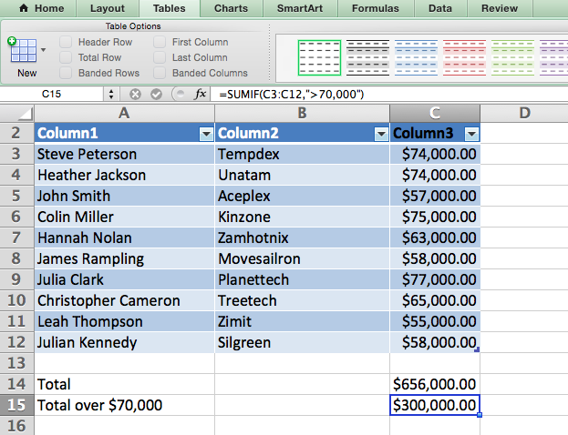
The SUMIF formula in Excel is denoted =SUMIF(range, criteria, [sum range]). This will return the sum of the values within a desired range of cells that all meet one criterion. For example, =SUMIF(C3:C12,”>70,000″) would return the sum of values between cells C3 and C12 from only the cells that are greater than 70,000.

Let’s say you want to determine the profit you generated from a list of leads who are associated with specific area codes, or calculate the sum of certain employees’ salaries — but only if they fall above a particular amount. Doing that manually sounds a bit time-consuming, to say the least.

With the SUMIF function, it doesn’t have to be — you can easily add up the sum of cells that meet certain criteria, like in the salary example above.

• The formula: =SUMIF(range, criteria, [sum_range])
  
  • Range: The range that is being tested using your criteria.
  • Criteria: The criteria that determine which cells in Criteria_range1 will be added together
  • [Sum_range]: An optional range of cells you’re going to add up in addition to the first Range entered. This field may be omitted.

In the example below, we wanted to calculate the sum of the salaries that were greater than $70,000. The SUMIF function added up the dollar amounts that exceeded that number in the cells C3 through C12, with the formula =SUMIF(C3:C12,”>70,000″).

12. TRIM

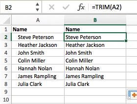
The TRIM formula in Excel is denoted =TRIM(text). This formula will remove any spaces entered before and after the text entered in the cell. For example, if A2 includes the name ” Steve Peterson” with unwanted spaces before the first name, =TRIM(A2) would return “Steve Peterson” with no spaces in a new cell.

Email and file sharing are wonderful tools in today’s workplace. That is, until one of your colleagues sends you a worksheet with some really funky spacing. Not only can those rogue spaces make it difficult to search for data, but they also affect the results when you try to add up columns of numbers.

Rather than painstakingly removing and adding spaces as needed, you can clean up any irregular spacing using the TRIM function, which is used to remove extra spaces from data (except for single spaces between words).

• The formula: =TRIM(text).
  • Text: The text or cell from which you want to remove spaces.

Here’s an example of how we used the TRIM function to remove extra spaces before a list of names. To do so, we entered =TRIM(“A2”) into the Formula Bar, and replicated this for each name below it in a new column next to the column with unwanted spaces.

Below are some other Excel formulas you might find useful as your data management needs grow.

13. LEFT, MID, and RIGHT

Let’s say you have a line of text within a cell that you want to break down into a few different segments. Rather than manually retyping each piece of the code into its respective column, users can leverage a series of string functions to deconstruct the sequence as needed: LEFT, MID, or RIGHT.

LEFT

• Purpose: Used to extract the first X numbers or characters in a cell.
• The formula: =LEFT(text, number_of_characters)
  
  • Text: The string that you wish to extract from.
  • Number_of_characters: The number of characters that you wish to extract starting from the left-most character.

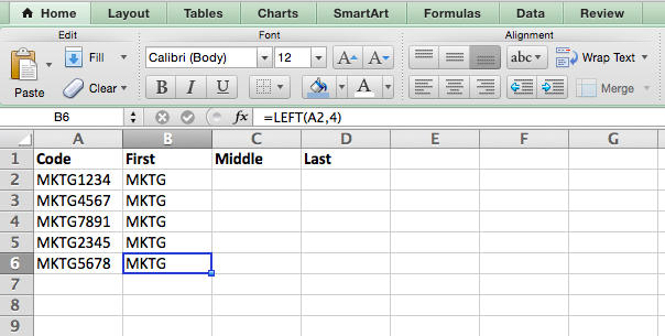
In the example below, we entered =LEFT(A2,4) into cell B2, and copied it into B3:B6. That allowed us to extract the first 4 characters of the code.

MID

• Purpose: Used to extract characters or numbers in the middle based on position.
• The formula: =MID(text, start_position, number_of_characters)
  
  • Text: The string that you wish to extract from.
  • Start_position: The position in the string that you want to begin extracting from. For example, the first position in the string is 1.
  • Number_of_characters: The number of characters that you wish to extract.

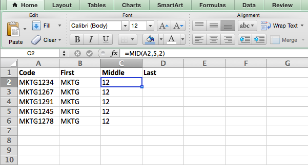
In this example, we entered =MID(A2,5,2) into cell B2, and copied it into B3:B6. That allowed us to extract the two numbers starting in the fifth position of the code.

RIGHT

• Purpose: Used to extract the last X numbers or characters in a cell.
• The formula: =RIGHT(text, number_of_characters)
  
  • Text: The string that you wish to extract from.
  • Number_of_characters: The number of characters that you want to extract starting from the right-most character.

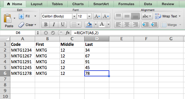
For the sake of this example, we entered =RIGHT(A2,2) into cell B2, and copied it into B3:B6. That allowed us to extract the last two numbers of the code.

14. VLOOKUP

This one is an oldie, but a goodie — and it’s a bit more in depth than some of the other formulas we’ve listed here. But it’s especially helpful for those times when you have two sets of data on two different spreadsheets, and want to combine them into a single spreadsheet.

My colleague, Rachel Sprung — whose “How to Use Excel” tutorial is a must-read for anyone who wants to learn — uses a list of names, email addresses, and companies as an example. If you have a list of people’s names next to their email addresses in one spreadsheet, and a list of those same people’s email addresses next to their company names in the other, but you want the names, email addresses, and company names of those people to appear in one place — that’s where VLOOKUP comes in.

Note: When using this formula, you must be certain that at least one column appears identically in both spreadsheets. Scour your data sets to make sure the column of data you’re using to combine your information is exactly the same, including no extra spaces.

• The formula: VLOOKUP(lookup value, table array, column number, [range lookup])
  • Lookup Value: The identical value you have in both spreadsheets. Choose the first value in your first spreadsheet. In Sprung’s example that follows, this means the first email address on the list, or cell 2 (C2).
  • Table Array: The range of columns on Sheet 2 you’re going to pull your data from, including the column of data identical to your lookup value (in our example, email addresses) in Sheet 1 as well as the column of data you’re trying to copy to Sheet 1. In our example, this is “Sheet2!A:B.” “A” means Column A in Sheet 2, which is the column in Sheet 2 where the data identical to our lookup value (email) in Sheet 1 is listed. The “B” means Column B, which contains the information that’s only available in Sheet 2 that you want to translate to Sheet 1.
  • Column Number: The table array tells Excel where (which column) the new data you want to copy to Sheet 1 is located. In our example, this would be the “House” column, the second one in our table array, making it column number 2.
  • Range Lookup: Use FALSE to ensure you pull in only exact value matches.
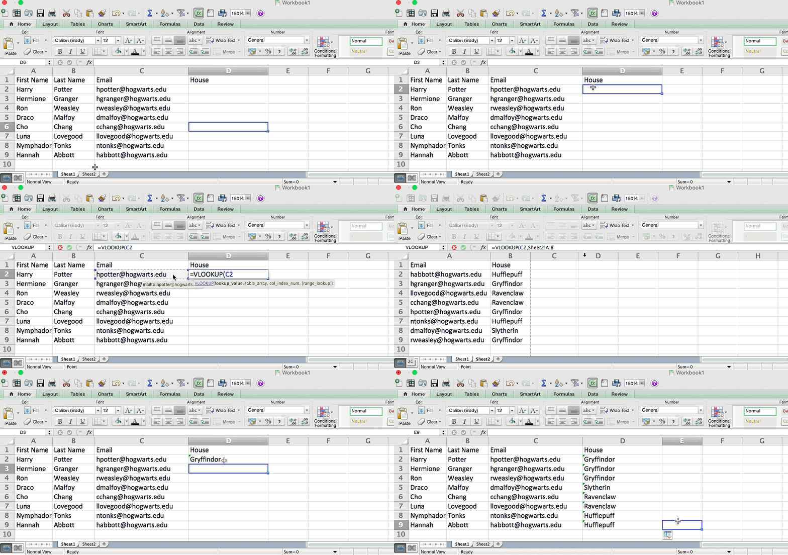
• The formula with variables from Sprung’s example below: =VLOOKUP(C2,Sheet2!A:B,2,FALSE)

In this example, Sheet 1 and Sheet 2 contain lists describing different information about the same people, and the common thread between the two is their email addresses. Let’s say we want to combine both datasets so that all the house information from Sheet 2 translates over to Sheet 1. Here’s how that would work:

15. RANDOMIZE

There’s a great article that likens Excel’s RANDOMIZE formula to shuffling a deck of cards. The entire deck is a column, and each card — 52 in a deck — is a row. “To shuffle the deck,” writes Steve McDonnell, “you can compute a new column of data, populate each cell in the column with a random number, and sort the workbook based on the random number field.”

In marketing, you might use this feature when you want to assign a random number to a list of contacts — like if you wanted to experiment with a new email campaign and had to use blind criteria to select who would receive it. By assigning numbers to said contacts, you could apply the rule, “Any contact with a figure of 6 or above will be added to the new campaign.”

• The formula: RAND()
  • Start with a single column of contacts. Then, in the column adjacent to it, type “RAND()” — without the quotation marks — starting with the top contact’s row.
• For the example below: RANDBETWEEN(bottom,top)
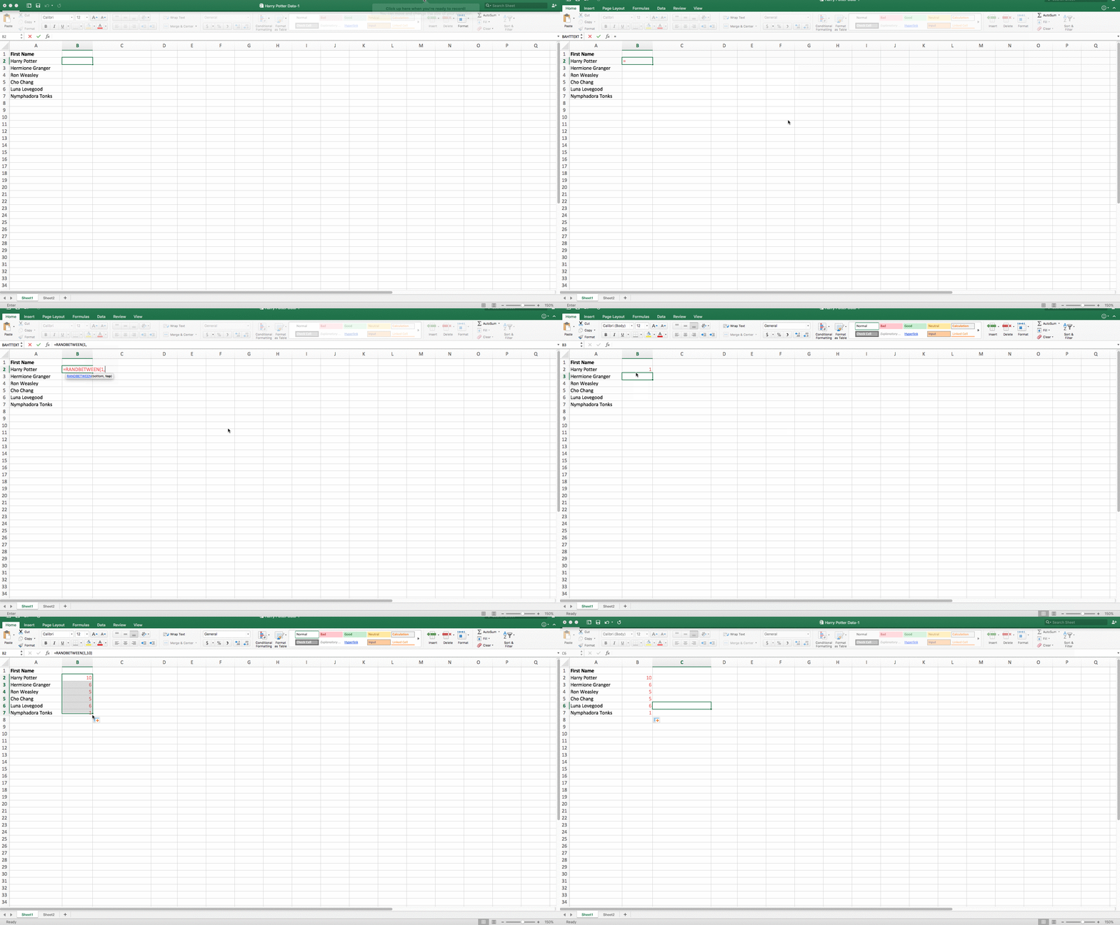
  • RANDBETWEEN allows you to dictate the range of numbers that you want to be assigned. In the case of this example, I wanted to use one through 10.
  • bottom: The lowest number in the range.
  • top: The highest number in the range,
• Formula in below example: =RANDBETWEEN(1,10)

Helpful stuff, right? Now for the icing on the cake: Once you’ve mastered the Excel formula you need, you’ll want to replicate it for other cells without rewriting the formula. And luckily, there’s an Excel function for that, too. Check it out below.

Sometimes, you might want to run the same formula across an entire row or column of your spreadsheet. Let’s say, for example, you have a list of numbers in columns A and B of a spreadsheet and want to enter individual totals of each row into column C.

Obviously, it would be too tedious to adjust the values of the formula for each cell so you’re finding the total of each row’s respective numbers. Luckily, Excel allows you to automatically compete the column; all you have to do is enter the formula in the first row. Check out the following steps: 

1. Type your formula into an empty cell and press “Enter” to run the formula.
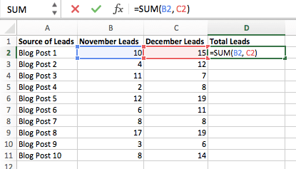
2. Hover your cursor over the bottom-right corner of the cell containing the formula. You’ll see a small, bold “+” symbol appear.
3. While you can double-click this symbol to automatically fill the entire column with your formula, you can also click and drag your cursor down manually to fill only a specific length of the column.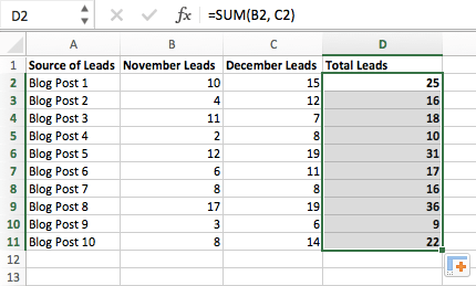Once you’ve reached the last cell in the column you’d like to enter your formula, release your mouse to copy the formula. Then, simply check each new value to ensure it corresponds to the correct cells.

Excel Keyboard Shortcuts

1. Quickly select rows, columns, or the whole spreadsheet.

Perhaps you’re crunched for time. I mean, who isn’t? No time, no problem. You can select your entire spreadsheet in just one click. All you have to do is simply click the tab in the top-left corner of your sheet to highlight everything all at once.

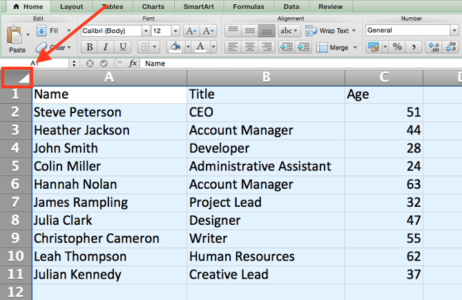
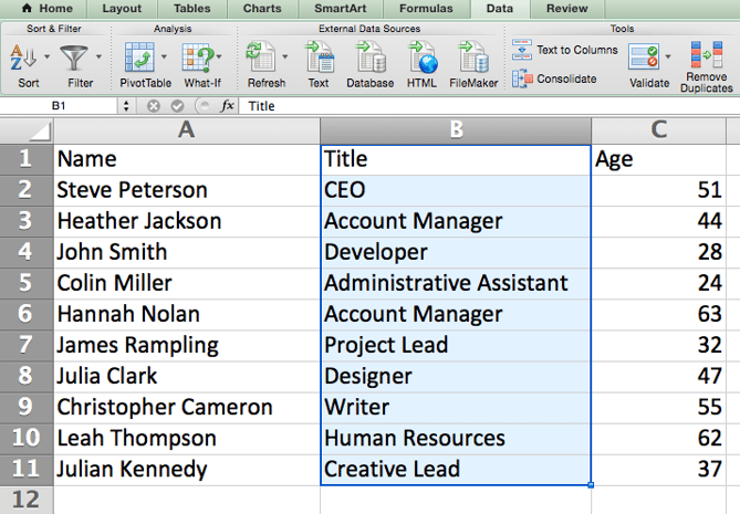
Just want to select everything in a particular column of row? That’s just as easy with these shortcuts:

For Mac:

• Select Column = Command + Shift + Down/Up
• Select Row = Command + Shift + Right/Left

For PC:

• Select Column = Control + Shift + Down/Up
• Select Row = Control + Shift + Right/Left

This shortcut is especially helpful when you’re working with larger data sets, but only need to select a specific piece of it.

2. Quickly open, close, or create a workbook.

Need to open, close, or create a workbook on the fly? The following keyboard shortcuts will enable you to complete any of the above actions in less than a minute’s time.

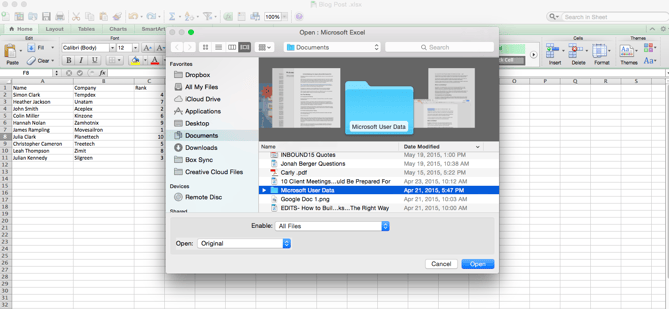
For Mac:

• Open = Command + O
• Close = Command + W
• Create New = Command + N

For PC:

• Open = Control + O
• Close = Control + F4
• Create New = Control + N

3. Format numbers into currency.

Have raw data that you want to turn into currency? Whether it be salary figures, marketing budgets, or ticket sales for an event, the solution is simple. Just highlight the cells you wish to reformat, and select Control + Shift + $.

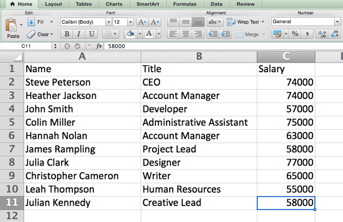
The numbers will automatically translate into dollar amounts — complete with dollar signs, commas, and decimal points.

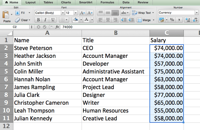
Note: This shortcut also works with percentages. If you want to label a column of numerical values as “percent” figures, replace “$” with “%”.

4. Insert current date and time into a cell.

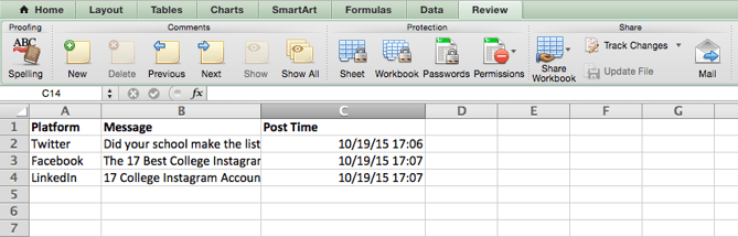
Whether you’re logging social media posts, or keeping track of tasks you’re checking off your to-do list, you might want to add a date and time stamp to your worksheet. Start by selecting the cell to which you want to add this information.

Then, depending on what you want to insert, do one of the following:

• Insert current date = Control + ; (semi-colon)
• Insert current time = Control + Shift + ; (semi-colon)
• Insert current date and time = Control + ; (semi-colon), SPACE, and then Control + Shift + ; (semi-colon).

Other Excel Tricks

1. Customize the color of your tabs.

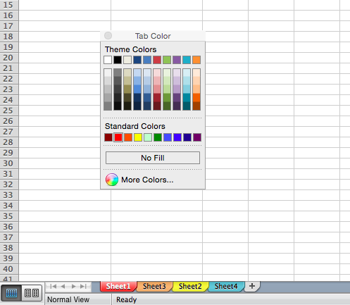
If you’ve got a ton of different sheets in one workbook — which happens to the best of us — make it easier to identify where you need to go by color-coding the tabs. For example, you might label last month’s marketing reports with red, and this month’s with orange.

Simply right click a tab and select “Tab Color.” A popup will appear that allows you to choose a color from an existing theme, or customize one to meet your needs.

2. Add a comment to a cell.

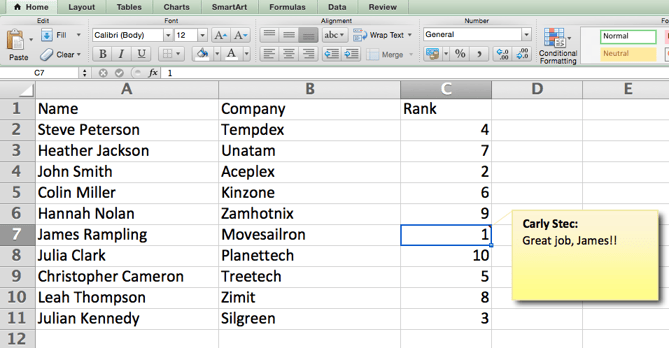
When you want to make a note or add a comment to a specific cell within a worksheet, simply right-click the cell you want to comment on, then click Insert Comment. Type your comment into the text box, and click outside the comment box to save it.

Cells that contain comments display a small, red triangle in the corner. To view the comment, hover over it.

3. Copy and duplicate formatting.

If you’ve ever spent some time formatting a sheet to your liking, you probably agree that it’s not exactly the most enjoyable activity. In fact, it’s pretty tedious.

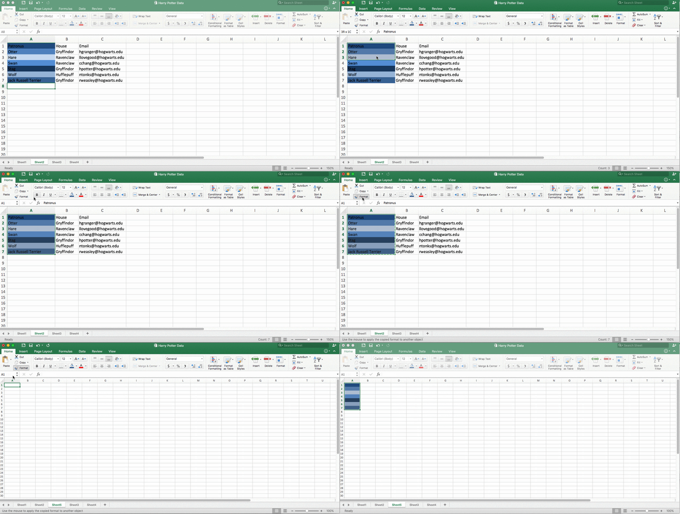
For that reason, it’s likely that you don’t want to repeat the process next time — nor do you have to. Thanks to Excel’s Format Painter, you can easily copy the formatting from one area of a worksheet to another.

Select what you’d like to replicate, then select the Format Painter option — the paintbrush icon — from the dashboard. The pointer will then display a paintbrush, prompting you to select the cell, text, or entire worksheet to which you want to apply that formatting, as shown below:

4. Identify duplicate values.

In many instances, duplicate values — like duplicate content when managing SEO — can be troublesome if gone uncorrected. In some cases, though, you simply need to be aware of it.

Whatever the situation may be, it’s easy to surface any existing duplicate values within your worksheet in just a few quick steps. To do so, click into the Conditional Formatting option, and select Highlight Cell Rules > Duplicate Values

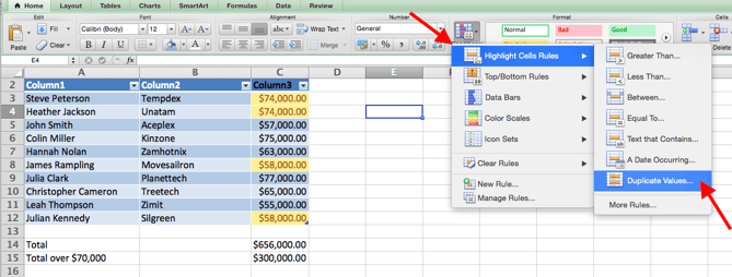
Using the popup, create the desired formatting rule to specify which type of duplicate content you wish to bring forward.

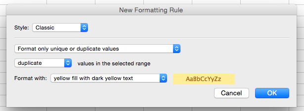
In the example above, we were looking to identify any duplicate salaries within the selected range, and formatted the duplicate cells in yellow.

In marketing, the use of Excel is pretty inevitable — but with these tricks, it doesn’t have to be so daunting. As they say, practice makes perfect. The more you use these formulas, shortcuts, and tricks, the more they’ll become second nature.

To dig a little deeper, check out a few of our favorite resources for learning Excel. Want more Excel tips? Check out this post on how to create a pivot table with medians.

When I studied abroad in Scotland last year, murmurs about the best restaurant in town echoed throughout my dorm complex all semester long. The joint was called Noodles & Dumplings, and despite its bland name, its cuisine was rumored to be packed full of flavor.

Naturally, once I heard about Noodles & Dumplings, I immediately bolted out of my dorm, power-walked down the cobblestone streets of my town, and burst through the front door of the restaurant. I was ready to gobble up all the shrimp fried rice I could possibly buy.

But after I placed my order and handed the cashier my credit card, she said something that turned my growling-stomach hunger into utter disappointment:

“We only take cash.”

As someone who never carries cash, eating my dinner that day required a jog to the ATM and a withdrawal of $200 to justify the hefty international ATM fee. It was quite a large commitment for some fried rice.

Now, I’ll be honest, the dish was delicious. It was definitely all that it was cracked-up to be. But was it worth the hassle? I probably wouldn’t be venting about this experience if it was.

Nowadays, your customers expect you to accept credit card as a form of payment, regardless of the size of your business. In fact, 77% of consumers prefer using credit or debit cards as their main form of payment. If you only accept cash, you risk losing a ton of customers — and revenue.

With this in mind, owning a POS system is crucial for your retail store’s or restaurant’s success. But POS systems aren’t just important because they can accept credit cards. POS systems can also track your inventory, measure your sales, and transfer funds to your bank account. It’s like a smart cash register that can help you better manage your business.

To help you pick the right POS system for your company, we’ve put together a list of the best ones for retail stores and restaurants. Read on to find the best POS system for your business.

What Is a POS System?

A point of sale (POS) system is a hardware and software system that lets you check customers out and accepts multiple forms of payment, like cash, credit cards, and mobile payments. POS systems’ hardware can print receipts, scan barcodes, and store cash. POS systems’ software can track inventory, measure sales, and transfer funds to your business’ bank account.

5 of the Best POS Systems for Retail & Restaurants

1. Square Point of Sale

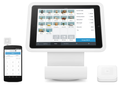
Image Credit: Square

Trusted by more than two million businesses across the globe, Square POS is an intuitive point of sale system that can keep tabs on your customers’ purchase history, send digital receipts, collect customer feedback, generate sales reports for specific products, and track your inventory. Square POS can also accept cards, cash, checks, and gift cards and transfer your funds to your bank account within one business day.

2. Toast

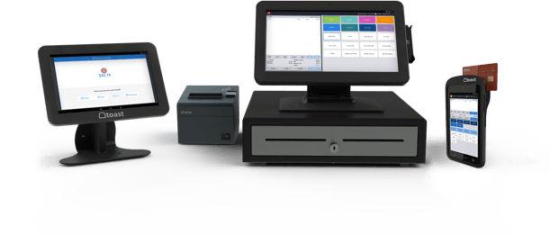
Image Credit: Toast

Tailored specifically to restaurants, Toast is an all-in-one point of sale system that can gather data on your food cost percentage, recipe costs, inventory variance, and menu engineering. It can also generate sales reports, sync your in-store and online menu so you don’t have to make the same changes multiple times, and has a built-in CRM that can collect your customers’ contact information and order history.

3. Shopify Point of Sale

Image Credit: Shopify

Shopify, the leading eCommerce platform, sells a point of sale system that can seamlessly integrate with your online Shopify store. In their POS system, each new order automatically creates a customer profile that includes their contact information, order history, and shopping habits.

You can also organize your products by category, type, season, sale, vendor, price, and inventory level. If you want to analyze your store’s performance, you’ll have access to a robust set of product reports, retail reports, and a dashboard.

4. Aloha

Image Credit: Aloha

Used by more than 80,000 restaurants around the world, Aloha is a single point of sale platform on which most servers and cashiers in the restaurant industry have been trained. With Aloha, you can let your customers order from their table, self-ordering kiosks, or even their mobile devices. You can also offer them promotions, rewards, and gift cards and generate reports about operational, sales, and employee data.

5. Vend

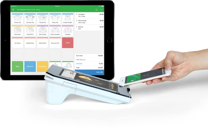
Image Credit: Vend

Designed for retail stores of all sizes, Vend is a smart point of sale system that more than 20,000 business trust and use every day. With Vend, you can keep track of your customers’ shopping habits in their customer database, measure your store’s performance, and manage inventory across multiple stores. Vend also integrates seamlessly with common business applications, like Shopify, Xero, PayPal, Apple, Worldpay, and Square.

On day one of my first internship during college, I was given a brief, 20-minute rundown on how the organization was structured, and what my role entailed, from my boss. I was then placed in a cubicle and given my first assignment. I got to work, though I felt both largely unprepared and frustratingly secluded.

Who was on my team? Wasn’t I supposed to meet them? Were there other interns, and where were they? And what’s the culture like, really?

Granted, it was an internship, but nonetheless, it quickly taught me the importance of onboarding.

According to an infographic by O.C. Tanner, 69% of employees are more likely to stay with a company for at least three years after a great onboarding experience.

Ultimately, your onboarding experience is your employees’ initial introduction to the company — if you don’t implement a memorable and helpful onboarding process that fully integrates new employees into your company, you risk higher turnover rates and less productive teams.

To ensure your new hires remain thrilled by your company and engaged in their roles long after the initial onboarding process, take a look at our onboarding checklists.

Onboarding Checklist

An onboarding checklist is one of the easiest ways to ensure your onboarding process includes all the necessary elements to fully integrate new employees into your company. However, it’s important to note, onboarding isn’t one-size-fits-all — a junior copywriter is going to need different tools to succeed at your company than a new marketing director.

While onboarding will vary for each employee, there are a few components you should include for any new hire.

The following onboarding checklists are for managers or HR departments to use when they are helping a new hire integrate into the company. Of course, certain tasks, such as necessary paperwork or required reading, will differ depending on the company or role.

Before The First Day: 

1. Acquire necessary paperwork (W-4, I-9, Insurance forms, Direct Deposit forms)

2. Ask new hire to review company employee handbook, and sign non-disclosure agreement

3. Prepare a workstation for your new hire 

4. Gather necessary tools, including technology such as a computer, and/or access to required software (i.e. Photoshop)

5. Provide new hire with company email 

6. Give new hire reading material, including company-wide policies and procedures, an organization chart, and a description of her role, as well as the company’s values, mission, and culture (unless this is included in employee handbook)

Before the first day, you might also consider leaving a note on your new hire’s desk, welcoming her to the team. Or, perhaps you can put branded material, like a sweatshirt or mug, on her desk as a welcome gift.

Additionally, consider sending your new hire an email, cc’ing all team members, welcoming her to the team.

On The First Day: 

1. Provide new hire with all necessary information, including dress code, where she can park, what time she should arrive, and what she should bring

2. Prepare team ahead of time — let them know the new hire is arriving, so they can greet her when she gets to her workstation

3. Reserve time on your team’s calendar for a “Welcome” lunch for the new hire, and tell the new hire ahead of time

4. Give your new hire a tour of the office, including bathrooms, kitchen, and support desk

5. Set up a 1:1 between manager and employee, so manager can explain what is expected of the new hire, how the department is structured, and answer questions the new hire might have

6. Assign the new hire a mentor, and ask mentor to set up a time to have lunch with the new hire

7. Give new hire a “30-day plan”, with reading material and important information regarding what is expected of her first month on the team

The first day will vary depending on how many new hires your company onboards at one time — one new hire, of course, will require a different process than a group of 30.

However, it’s important you keep the new hire busy and engaged. You don’t want the new hire to feel awkward sitting at her desk waiting for instruction. You want to demonstrate you’ve taken the time to plan a full, productive day for the new hire.

To keep the employee engaged and excited, you might give her a “30-day plan”. Among other things, the first month plan can include:

• Names of people you suggest she reach out to for lunch or coffee. These are likely people she’ll be working with closely, or people you believe can offer her guidance
• Reading material that will help her succeed in her new role — if she’s the new social media manager, perhaps you can include blog posts about social media you’d like her to read
• The manager’s expectations for her first month (i.e. “I’d like you to brainstorm and present one marketing video campaign idea by the end of this month”)

During Week One:

1. Consider asking both new hire and manager to take the DiSC, if they haven’t already — understanding work personalities can help 1:1’s go more smoothly

2. Have 1:1 with manager and new hire, in which manager explains how she expects 1:1’s to go, and how she wants new hire to prepare for each 1:1 meeting

3. Within first few days, assign the first project to your new hire. This will help her feel like a valuable asset to the team, and allow her to become more comfortable in her role

4. Ensure all required paperwork is filled out

5. Review employee performance evaluations, and set goals for month one

6. If necessary, set aside time to teach new hire how to use new software 

As a manager, it’s critical you clear your schedule (for the most part), if you’re solely in charge of your new hire’s integration into the new team. Take the time to thoughtfully consider one-on-one lessons you can set up to acclimate your new hire to your software or work processes.

Additionally, keep her engaged in what’s happening with the larger team. Ask her if she wants to sit in on meetings that, while not directly relevant to her at the moment, might be useful to her as she grows in her role — or simply might help her get a better sense of what your team does, or what kind of culture your department fosters. 

Ultimately, it’s critical she has a firm understanding not just of her own role, but how her role fits into the company as a whole.

For the First Month: 

1. Set up weekly meetings to give your new hire constructive criticism regarding her first couple assignments 

2. Provide her with additional reading material as you see fit — perhaps you suggest books related to her role, or articles you feel will help with her professional growth

3. Check-in that she is meeting the appropriate people and getting lunch or coffee with core members of the team

4. Ask for feedback from the new hire(s) — if its a large group, offer the option to fill-out an anonymous survey. If you have only one new hire, simply ask her what else she needs to succeed or what she wishes the company provided 

5. Organize a team outing to help the new hire bond with the team — if dinner is difficult to plan, consider getting lunch with the team away from the office

6. Ask her mentor to check-in with her

During the first month, it’s important your employee have a firm understanding of what’s expected of her, and who she can turn to for guidance.

Additionally, your new hire likely has particular preferences regarding how she’d like to be managed. After providing constructive feedback during each one-on-one, ask her if she has any feedback for you as her manager.

Towards the end of the initial onboarding process, ask new hires to fill out a survey regarding the onboarding process. Your HR team can use these suggestions to alter the process for future employees.

While we’ve only covered the first month, it’s important to note studies have shown companies with less than one month dedicated to onboarding are 9% less likely to keep first-year employees than companies with longer processes. Your new hires need time to fully acclimate to their roles and the company culture. A good time frame is roughly one to three months minimum, but some companies choose to implement an onboarding process that lasts a full year.

Ultimately, a good onboarding process will take into consideration both what your team needs from your new hire, and what your new hire needs to succeed in her role. It might require flexibility and patience, but it’s worth it if you can show your new hire she’s a valuable asset to your team. You can also adjust your strategies as you learn more about her strengths and weaknesses. 

One of the most frequent questions we get from aspiring and current inbound marketers is, “How do you manage all of that content?”

When we tell them we use an editorial calendar, the next question is often, “Oh, how much does that cost?”

Nothing. Because, for the most part, we use Google Calendar.

Download our free editorial calendar templates for Google Calendar and Microsoft Excel here.

Surprised? There are a lot of great calendar tools out there you can choose from. (In fact, for those of you who are HubSpot customers, there’s a marketing calendar built right into HubSpot’s software.) But after trying a ton of other solutions, our team found that we really operated the best with just a simple Google Calendar. In fact, this has actually been the longest-running editorial calendar solution our team has ever seen.

Here’s how we set it up.

How to Create a Blog or Editorial Calendar in Google Calendar [Excel Template]

Step 1: Click here to download our free editorial calendar templates.

First thing’s first: Download the calendar templates, above (they’re free.) By doing this, you’ll have three editorial calendar templates on your computer to use at your leisure: one for Google Calendar, one for Excel, and one for Google Sheets. In this blog post, we’ll be going over how to import the Excel template into Google Calendar.

By default, the publish dates on the templates you download will be stamped for the year 2016. Feel free to change them to the present year in the spreadsheet itself — you can also drag them to the dates of your choosing after you upload the file into Google Calendar.

Step 2. Import Excel into Google Calendar.

Google Calendar makes it easy to load a calendar you might have pre-created in another program into Google. This includes Microsoft Excel. Here’s how to import the Excel calendar template you downloaded in the previous step into Google Calendar:

1. Open Google Calendar.

Once you’ve downloaded (or, for that matter, created) a calendar that opens in Microsoft Excel, it’s time to open Google Calendar. Just make sure you’re already logged into the Gmail account you want this calendar to give access to.

2. Use the lefthand dropdown menu to create a new calendar.

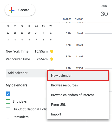
Now it’s time to set up your Google Calendar to accommodate the information in your Excel spreadsheet. First, go into your Google Calendar and click the three vertical dots to the right of “Add calendar,” as shown in the screenshot below. In the dropdown menu that appears, select “New calendar.”

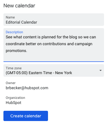
3. Fill out the details of your new calendar.

Fill out the fields that appear on the next screen. This includes a brief description of your calendar, as shown below, to give people proper context when you invite them into this calendar. When you’re done filling in the details, click “Create calendar.”

4. Import your XLS or CSV file from the same dropdown menu.

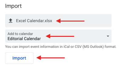
Using the same dropdown menu you used to create your editorial calendar, you’ll now import the Excel file itself into Google Calendar. Click those vertical three dots next to “Add calendar,” and select “Import.”

Click the upload box that reads “Select file from your computer,” and locate the file entitled “Blog Editorial Calendar – Excel” that was included in the ZIP file you downloaded in Step 1, above.

5. Select which calendar to add this file to.

In the second box below your imported file, click the “Add to calendar” dropdown. Be sure to choose the name of the calendar you just created from the dropdown menu, as shown below. Then, click “Import.”

6. Click Import.

Once you’ve uploaded your Excel file and selected the calendar you want to add this file to, click “Import.” You should see an Import calendar dialog box telling you that seven events were successfully imported. Click “Close.”

Now, if you didn’t change the dates of the first seven assignments in the original Excel document, you can now. Navigate to January 3, 2016, which is the start of your calendar. Be sure all of your other calendars are temporarily hidden by clicking the colored box to the left of the calendar name. On the week of January 3, 2016, you should just see one “Blog TBD” calendar event on each day from 10 a.m. to 11 a.m.

Use the edit window of each assignment to change the publish date. For example, if you’re satisfied with the 10 a.m. publish time, you can simply change the date from January X, 2016 to January X, 2019. Each assignment will then appear as event blocks in your 2019 monthly calendar view.

Step 3: Determine your publishing schedule.

Now that you have your calendar created, it’s time to fill it in with assignments for the year. This is when you have to make some decisions about your blog’s publishing schedule.

While the Excel file you imported accounts for one blog post per day, this doesn’t mean you need to publish seven days a week. Maybe you want to publish every Monday, Wednesday, and Friday. Or perhaps you plan on publishing on just Thursdays. Remember, the key to successful blogging is quality over quantity. Don’t overcommit to a blogging schedule if the quality of your content will take a hit. (Read this blog post for some great benchmark data on how often companies should blog.)

If you decide to decrease the number of days you want to publish, click on the calendar event of that day and select “Delete.”

Even if you wanted to publish multiple times a day, updating this calendar is as easy as adding an event. Select a slot on your calendar to add another “Blog TBD” event and copy the default description from another one of the events you imported.

Next, it’s time for some minor adjustments. Currently, the “Blog TBD” events are set for 10 a.m. Feel free to move these events to whichever time your blog publishes during the day. (Curious about what time is best for you to publish a blog post? Read this how-to blog post to learn how to create a Custom Google Analytics Report.)

Step 4: Set up recurring events.

Now that you have your publish dates and times set, you can make these recurring events on your calendar. If you have a regular publishing schedule, like every Monday, Wednesday, and Friday at 10:00 a.m., then put that in as a recurring “slot” on your calendar. It’s okay if you don’t have a piece of completed content — or even a working title — to put there yet. It’s just a reminder that you want to publish something that day.

To add your recurring slot, click on your first “Blog TBD” event and click the pencil icon to edit your event. This will take you to the details of the post, where you can create a custom recurring schedule for each assignment, as shown in the screenshot below.

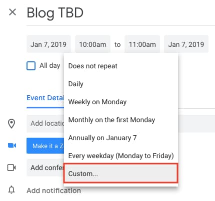You can set the post up as a recurring post so it automatically appears every Monday, Wednesday, and Friday at 10:00 a.m. (or whatever days and times you want).

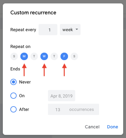
Once you’ve selected the recurring days, hit “Done” and “Save,” and you’ll have an editorial calendar framework to work with.

For now, keep the title of the event as “Blog TBD,” but feel free to customize the description with any extra details you want to be sure you include for each post. Wait to invite any guest, as we’ll use this to assign posts to an author once you begin filling in your topics. With everything complete, click “Save.”

If you don’t have a recurring schedule like this, you might not be in need of an editorial calendar just yet — but it is a good way to set goals for yourself. If you know you want to publish a certain number of posts each week, even if you don’t hit every single slot, it’s a good reminder for yourself and your team that this is something you should all be striving for.

Step 5: Fill your publishing slots.

Now that you know all of the slots you want to fill, you gotta actually … you know … fill ’em. (If you don’t have topic ideas yet, check out this free topic idea generator. It’ll give you some good ideas for content to put in the calendar.)

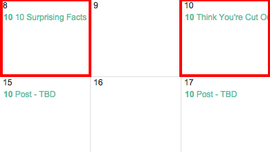
Let’s say one of the posts you want to write is “10 Surprising Facts About Tapirs,” and one of the posts you’ve already written and want to publish later is “Think You’re Cut Out to Own a Tapir? Read This First.” Cool! Just add ’em both to the calendar by clicking on “Post – TBD” on the correct date, choosing “Edit Event,” and then changing the “Post – TBD” text to the actual title of the post.

Now, let’s say you don’t actually want to write “10 Surprising Facts About Tapirs,” and you want your colleague to write it instead. To assign the post an author, you’ll invite them to the event as a guest. To do this, click on the event, hit “Edit Event,” then invite that colleague to the post by typing his or her name or email address into the “Add guests” box, selecting “Add” when their name pops up, and hitting “Save” on the event once you’re done.

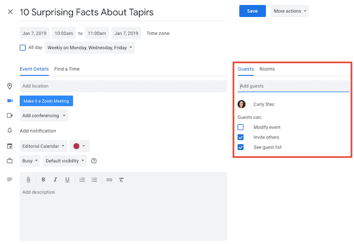
Now, anyone can see who is responsible for writing the post that’s going up in that time slot.

You can take it a step further by adding details to the “Description” box of the event, as shown in the large box in the screenshot above. You might include a quick synopsis, the keywords you plan to target the post for, the target audience you’re trying to reach, and the offer or CTA you will direct the reader to at the end of the post. Don’t forget a due date for the draft.

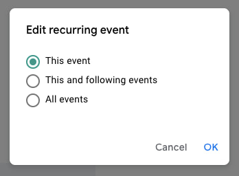
Before Google Calendar will let you save the event, you’ll see a dialog box asking if you would like to change just this event or all of the events in the series. Select “Only this event.”

Repeat these steps to assign each blog topic today and in the future.

Step 6: Share your editorial calendar with others.

Now that you have your calendar set up, you can start to invite people to see it. I’d recommend you start with your immediate team and regular contributors — as well as anyone who regularly asks you about publishing content on your company blog.

To share this editorial calendar with people, simply find your editorial calendar under “My Calendars,” as shown below. Click “Settings and sharing” when it appears in the dropdown arrow, and you’ll be taken to the same screen we saw when you first filled out the details of your editorial calendar in Step 2.

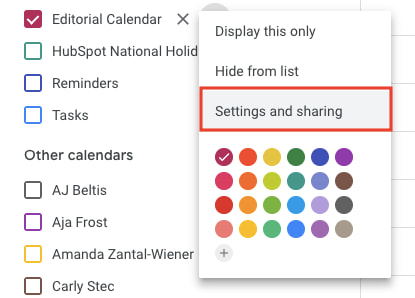Then, you can add in the names of people with whom you’d like to share the calendar and set the right permission levels for each invitee.

It’s wise to keep those with the permission settings to manage changes and sharing to a minimum so there aren’t too many cooks in the kitchen — but I recommend you let everyone see all event details so it’s clear exactly what content is going up in each slot.

Under the “Share with specific people” heading, enter the email addresses of those on your content team and decide if they have viewing, editing, or admin privileges. Save your updated settings.

Why Using Google Calendar as an Editorial Calendar Works

I mentioned earlier that we tried a lot of different editorial calendar solutions, and this is the only one that’s stuck for more than a couple months. I think one reason for that is because we use Gmail for our corporate email, which means everyone on our team is already in Gmail (and their calendar, specifically) all day. As a result, it isn’t hard for people to form a habit of checking the editorial calendar, because it’s not difficult for them to find it.

Google Calendar also makes things really easy to move around and schedule because … well … it’s already a calendar. It has all the functionality you need to schedule stuff out and let the people who need to know about it know. When we were using other solutions for this, we were trying to hack a calendaring function instead of just relying on one that already existed.

Along those lines, adding people to view your calendar is simple, which makes it easy for multiple teams to collaborate, see what’s being published, and figure out when they might be able to launch content and campaigns.

Finally, this sets a precedent for other teams to coordinate with you in a really simple way. You can have a calendar for upcoming campaigns, offers, social media pushes, product launches — you name it. And you can all share those calendars with one another for a single-screen view of everything that’s going on so you can coordinate more easily.

Are there other solutions of there for maintaining an editorial calendar? Of course. But if you’re looking for a minimum viable product, and a free one at that, this ain’t too shabby. It’s kept our content team sane, agile, and transparent for quite some time — and I think it could do the same for you.

In a world hooked on instant gratification, one of the worst things a brand can do is not give their audience what they want. If your website visitors see a 504 Gateway Timeout Error page when they’re looking for help or information to do their jobs better, they could get annoyed and lose trust in your brand, permanently damaging your reputation.

Unfortunately, 504 Gateway Timeout Errors are rather mysterious. They indicate what happened to your website, but they don’t tell you why it happened, making it challenging for you to pinpoint its cause and ultimately correct the issue.

To help you fix your 504 Gateway Timeout Error and avoid losing brand sentiment and trust, we’ve fleshed out exactly what the issue is and its most common solutions.

Image Credit: Cloudflare

Fortunately, there are five common and effective solutions for fixing most 504 Gateway Timeout Errors’ causes.

1. Look for server connectivity issues.

Most websites live on multiple servers or third-party hosting providers. If your server is down for maintenance or any other reason, your website could serve visitors a 504 Gateway Timeout Error page. The only way to troubleshoot this issue is to wait for your server to finish maintenance or fix the problem causing the error.

2. Check for any DNS changes.

If you’ve recently changed host servers or moved your website to a different IP address, it’ll make changes to your website’s DNS server. This could cause your website to serve its visitors a 504 Gateway Timeout Error page. Your website won’t be up and running until these DNS changes take full effect, which can take a few hours.

3. Sift through your logs.

Server logs will provide details about your server’s health and status. Sift through them to uncover any alarming information.

4. Fix faulty firewall configurations.

Your firewall is your website’s gatekeeper, protecting your site from malicious visitors or distributed denial-of-service (DDoS) attacks. Sometimes, a faulty firewall configuration will cause your firewall to deem requests from a content delivery network as an attack on your server and reject them, resulting in a 504 Gateway Timeout Error. Check your firewall configuration to pinpoint and fix the issue.

5. Comb through your website’s code to find bugs.

If there’s a mistake in your website’s code, your server might not be able to correctly answer requests from a content delivery network. Comb through your code to find bugs or copy your code into a development machine. It’ll perform a thorough debug process that will simulate the situation that your 504 Gateway Timeout Error occurred in and allow you to see the exact moment where things went wrong.

Workplace culture and strong internal relationships are undeniably critical for your company’s long-term success. Focusing your efforts on cultivating good relationships between employers and employees can help your Human Resources department mitigate conflict, build trust between team members, and decrease turnover rates.

At its core, employee relations is a branch of human resources that deals with policies regarding your employees’ relationships with their employers, and each other.

For instance, an employee relations manager might create and implement policies regarding sexual harassment in the workplace, negotiate new contracts as employees move up in the ranks, and work with directors or employers to create benefits packages for individuals or departments.

If you aren’t sure what employees relations is, or simply aren’t sure why it’s important, keep reading.

What is Employee Relations?

Riley Stefano, a Culture Content Creator at HubSpot, explains employee relations like this — “At its core, employee relations is about trust and transparency. But that doesn’t just happen overnight — you have to build it. And every department, team, manager, and leader is responsible for building and adding to that culture of trust and transparency. In People Operations, we strive to create remarkable experiences for employees throughout their time at HubSpot so that they can do their best work and help HubSpot grow better.”

Stefano goes on to say, “To cultivate strong employee relations, we have to have empathy. We have to listen, share information, take feedback seriously, and adapt with our employees to maintain long-lasting and trustworthy relationships with all of our employees globally.”

Essentially, employee relations is any effort or programming a company implements to ensure their employees are treated fairly, feel safe, and are happy in their work environment. Additionally, employee relations cannot be successful unless employees feel there is a level of transparency from management.

At HubSpot, this includes utilizing HR Business Partners, and implementing culture programming and events to help build stronger relationships with HubSpot employees.

However, employee relations programming might look different at your company. Perhaps your employee relations efforts include ensuring a good work-life balance for employees, or giving each employee stock in the company, so they are treated as stakeholders in the business.

Alternatively, perhaps you hire an employee relations manager to provide guidance on new and existing contracts and policies, so that you can ensure each employee is treated fairly and feels safe in the workplace. Perhaps your employee relations manager can also gather employee feedback, and use it to create new benefits packages that incentivize and properly reward employees for their hard work.

It’s critical you take the time and effort to ensure you’ve cultivated strong relationships between employers and employees. If your employees respect leadership, they’re more likely to work harder, communicate better, and feel more engaged at work. All of these things can motivate employees to go above-and-beyond in their roles. 

Ultimately, a company can’t be successful unless there’s a universal alignment of vision, goals, and purpose between employers and employees — and that alignment doesn’t happen naturally. It must be cultivated, in large part through strategic employee relations efforts.

Your visitors are bound to make the occasional mistake while completing your online forms. When it comes to shipping or registration forms, for example, there are a number of form fields a visitor is required to complete. And let’s face it, your visitor may not be thrilled about having to enter their address, credit card information, and more, and therefore, they may move through your form quickly. Chances are, some visitors will misspell something, type in an incorrect zip code, or miss a number in the credit card field.

You might be wondering how to ensure your visitors stay efficient and accurate so they aren’t wasting any of their own time trying to locate and correct their errors in your forms. You also may be wondering how to achieve this so you don’t waste any of your own time trying to work through incorrect or invalid information.

Enter: Error messages.

 

Why Are Error Messages Important?

Error messages play a large role in your visitors’ user experience. If someone is repeatedly unable to submit your form and has no idea why or what the issue is, there’s a large chance they’re going to feel frustrated, angry, or simply leave your site altogether.

By adding well-crafted error messages to your forms, your form will feel professional and thoughtful to your visitors. Most importantly, error messages will enhance your form’s user experience — and great user experience means you’re more likely to see a boost in conversions. It also means more happy customers who are likely to return to your site and become promoters for your business. 

To achieve a fantastic user experience, you can’t simply implement any error message in your forms. In fact, there are plenty of forms out there that include error messages that aren’t thoughtful or effective. In this post, we’ll cover some of the most frequently made error message mistakes.

Error Message Design: 6 Mistakes to Avoid and Good Examples to Follow

Let’s review six common mistakes you’ll want to avoid while creating error messages for your web forms and six preferable examples you can implement instead.

1. Error Message Placement

The placement of your error message is crucial. If someone submits your form and then sees a red box with the message “Your form contains errors” they wouldn’t actually know where the errors are located. Instead, avoid making your visitors feel confused by placing the message next to the error itself.

Mistake: Poor error message placement

Source

This is an example of unhelpful and vague error message placement. It would be exceptionally difficult for someone to automatically know the exact location of the error with such an unclear message located in a pop-up box.

Good example: Great error message placement

Source

This is called inline error message placement — it’s located directly inline with the error so your visitors are able to clearly see the issue at hand and quickly fix it.

2. Blame the User

Ever heard that saying, “The customer’s always right”?

Well, that same message applies to your web forms and their error messages. You should avoid any negative language and refrain from blaming your visitors for the error — use positive phrases and don’t place the blame anyone or anything.

Mistake: Blame the User 

The last thing you want to do is target your visitor and make them feel bad or belittled. Don’t ever blame them for the error in the form (even if they really did cause the issue). 

You should also avoid negative and vague phrases such as, “Oops!” or “Something went wrong.” Having to correct an error or two might be a frustrating process for a person in a rush or someone who has already worked through multiple other errors in the same form. And lets face it, negative language isn’t going to make your visitors excited about correcting their mistakes — it’s also simply not at all helpful.

Source

Good example: Don’t blame anyone or anything

Source 

In your error messages, you want to sound positive, calm, and straightforward. You should also avoid blaming anyone or anything. Inserting polite words and phrases such as “please” is also a nice and professional way to ask your visitors to correct their errors while also making a good impression.

3. Error Message Copy

Your error message copy (what the error message actually says) matters. Otherwise, how would your visitor understand what the error actually is or how to fix it? Using clear and direct language will help your visitors understand what caused their error in the first place and how they should go about correcting it.

Mistake: Lack of clarity

Source 

Although this error message is inline and shows the visitor there’s an issue with the email address they entered, simply saying the address is “invalid” isn’t helpful for visitors. In this scenario, how are visitors supposed to know if they misspelled their email address, if they need to try another email address, or if already have an account they forgot about (and need to head to the login page instead)?

Unclear and vague copy puts your visitors through a not-so-exciting and time-consuming guessing game.

Good example: Be clear and concise

Your message copy should not only be clear, concise, and explain the issue at hand, but it should also give the visitor simple directions on how to fix the error. This way, they stay productive and both your company and form feel professional and thoughtful.

4. Error Message Clarity

Error message copy is a great lead-in to a similar, common mistake: lack of error message clarity. Your message should be so clear that an elementary school student could understand it and know how to fix the error. 

To determine your error message’s level of clarity, you should take a look at your form field requirements. For example, if you have unclear requirements listed and an error message pops up on the form, your visitors are going to have a hard time understanding how they’re supposed to fix the issue .

Mistake: Not listing form field requirements

Source

If your form has password requirements yet you don’t clearly list them out anywhere, your visitor will most likely find it difficult to create a valid password. They’ll have to use the process of elimination to create a password successfully which could take a lot of time. Again, talk about an agitating process that your visitors simply don’t have the time for.

Good example: List form field requirements

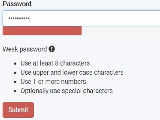
By clearly listing your form field requirements, such as your exact password requirements, you provide your visitors with a solution to avoid making any errors in your form. And if they do still make a mistake, they can quickly skim those requirements to learn how to amend the issue.

5. Concise Error Message Descriptions

While completing your form, it’s probably safe to assume your visitors aren’t going to want to sit around reading a long error message description. Reading wordy, long-winded descriptions about anything can feel confusing and tedious. To avoid this, your error message descriptions should briefly explain the precise actions your visitors can take to fix their mistake.

Mistake: Long, confusing error message descriptions

Source 

Long and confusing error message descriptions typically defeat the purpose of what you’re trying to do (which is help your visitor correct their error). In fact, they can make it significantly more difficult to uncover the real issue at hand and understand how to fix it.

Good example: Keep error messages straightforward

Source

When you explain the reason for your visitor’s error, be as straightforward and short as possible. Use language that points the visitor directly to their mistake and briefly explains how to fix it so they can make the correction on their own without any hesitation or confusion in a timely manner.

6. Obvious Error Messages

Making your error messages pop so they’re easy to see and read is a simple way to enhance UX (user experience). Make your error messages bright, bold, and obvious so your visitors can quickly correct their mistake and move on with their submission. To create an obvious error message, consider things like size, color, font, and other factors that contribute to the message’s overall appearance.

Mistake: Make the error message hard to see 

Source

Typically, error messages and warning signs are the color red — this error message example is green … which is a color that often signals success. You can see how this might lead to some puzzled visitors.

Using narrow and light-colored font on a white background is also slightly difficult to read. Additionally, the message’s action button, “OK”, stands out more than the word “ERROR” at the top of the summary box.  And “Error” is arguably the most important part of this message because it’s what actually tells visitors there’s an issue with their submission.

Good example: Make the error message easy to identify

Source

When creating your error message, use intuitive, error-related cues (such as the color red) to bring the mistake to your visitor’s attention. 

Some may say that a lot of bright red on a page could potentially overwhelm a visitor or make them feel targeted. But incorporating neutrals such as white or black, or even a faded or less-abrasive shade of red, helps bring balance to your message. This error message also uses warning signal icons that direct visitors to the locations in which errors exist, a readable font, and an easy-to-see action button that clearly states you can resubmit, or “Send”, your form again.

Back To You

Including well-crafted error messages in your web forms is a great way to enhance your user experience and, therefore, boost your conversions. There are a number of ways to avoid the most commonly made error message mistakes that may cause your visitors to feel frustrated, angry, or leave your site altogether. 

By incorporating the quick fixes to these mistakes, your forms will feel professional and thoughtful, initiating a positive relationship with your visitors that will keep them coming back to your site. So get started crafting great error messages today with these easy-to-implement guidelines that will improve your UX and increase your number of leads and conversions.

As a marketer, you need to record your computer screen more often than you’d think. Whether you’re teaching a new hire how to use a tool, explaining a complex project when an email just won’t do, or recording a personalized product demo, you need to know how to record your computer screen.

Fortunately, we’ve put together a quick and easy guide for recording your computer screen on a Mac and Windows 10. Read on to learn how to do so.

How to Record Your Screen on a Mac

Apple pre-installed QuickTime Player, an app that lets you record, edit, play, and share audio and video files, onto every Mac. You can use it to record your computer screen.

1. Open QuickTime Player by searching for it in Launchpad.

2. Once you’re in Quicktime, click “File” and select “New Screen Recording”.

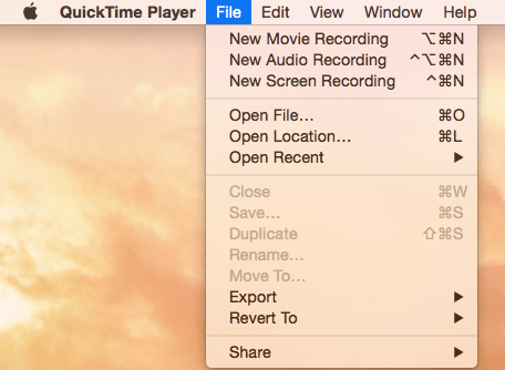
3. Press the downward facing arrow next to the “Record” button to choose the following recording options:

• Microphone: Choose “None” to record your screen with no sound. Choose “Built-in Microphone” to record your screen with sound.
• Options: Choose “Show Mouse Clicks in Recording” if you want your clicks to appear as a circle during your screen recording.

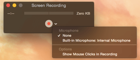
4. Click the “Record” button and choose one of the following recording types:

• Click your screen to record your entire computer screen.
• Drag a section of your screen that you want to record.

5. To finish recording, click the “Stop” button in the menu bar, which will be to the left of the “WiFi” button.

6. To save your recording, click “File”, press “Save”, and name your recording.

How to Record Your Screen on Windows 10

On Windows 10, Microsoft pre-installed the Xbox App, which has a built-in screen recorder that’s designed for recording video games on your computer. You can still use it to record your screen for marketing purposes, though.

1. Type “Xbox” into the search box and open up the app.

 

2. To open the Game Bar, which lets you record your screen, hold the “Windows” and “G” keys on your keyboard. Then, click “Yes, this is a game”.

Image Credit: Lifewire

3. To choose your screen recording’s quality setting, determine whether or not you want to record audio, or set a maximum clip length, open the “Game DVR” options in the Xbox app.

Image Credit: Lifewire

4. Click the “Record” button or hold the “Windows”, “Alt”, and “R” keys on your keyboard to start recording your computer screen.

Image Credit: Lifewire

5. Click the “Stop” button when you’re finished recording. Your recorded video will be saved in your “Videos/Capture” folder.

 

5 of the Best Free Screen Recorders for Mac and Windows

If you’d like to record your screen with more advanced tools that are still free, check out these five screen recording tools that you can download or access online.

1. OBS Studio

OBS Studio is an open source software for video recording and live streaming. Designed for gamers to record and stream themselves playing video games, OBS Studio offers advanced post-production tools, like customizable transitions, muting or turning on audio sources, and editing, which allows you to tinker on almost every aspect of your recording or broadcast.

Image Credit: Tech Radar

2. Apowersoft Free Online Screen Recorder

Apowersoft is a web-based screen recorder, so you don’t have to download it. By just visiting their website, you can record your screen for however long you want, pick a certain part of your screen to record, insert your webcam into your screen to talk about what exactly you’re doing, capture video and audio at the same time, and make annotations while recording.

Image Credit: Tech Radar

3. Debut Video Capture

Currently in public beta, Debut Video Capture isn’t as sleek as the other tools on this list, but it still has a similar level of functionality. With the tool, you can spotlight your cursor during your recordings, add captions to your recordings, adjust your recordings’ color and video effects, and customize the size and frame rate of your recordings.

Image Credit: Tech Radar

4. Icecream Screen Recorder

With support for over 50 languages, Icecream Screen Recorder is one of the best screen recorders for global teams. You can also add your own watermark to your recordings, choose your recordings’ video quality, trim recordings, and set timers for each task you want to complete during your screen recordings.

Image Credit: Lifewire

5. TinyTake

TinyTake is a more basic screen recorder, but you can still record your screen for up to two hours, email your screen recording to colleagues, and even create a shareable link of it.

Image Credit: Lifewire